Introduction to Artificial Neural Networks part three: Deep Learning & Reinforcement Learning

This post will cover the concept of deep learning and dive deeper into the reinforcement learning approach.

To get a better understanding of the material covered in this post I recommend reading the first two parts of this series. (Part 1, Part 2)

In 2016, the master player Lee Se-dol has managed to beat the AI system AlphaGo in one out of five games at the Chinese board game GO, but despite that, he has decided to retire from playing GO professionally stating that AI has reached a level where it can no longer be defeated by humans.

This was a huge achievement and true landmark in AI development for AlphaGo, which was trained using reinforcement learning and developed by DeepMind.

When IBMs Deep Blue beat Kasparov at chess most experts thought that  “yeah, but chess is easy! AI will never be able to master the game of GO”. Well this has happened and brings the question if what we think AI will never master today will actually be mastered sooner than we expect it.

With that in mind, let’s dive in and learn what deep learning is, how and why reinforcement learning works so well that it can beat humans at any given game we have invented.

DEEP LEARNING

Deep learning is a specialized form of machine learning that teaches machines to do what humans are naturally born with: learn by example.

Though the technology is often considered a set of algorithms and networks that aim to ‘mimic the brain’, a more appropriate description would be a set of algorithms and networks that ‘learn in layers’.

Neural network architectures are widely used in most deep learning methods, which is why deep learning models are often referred to as deep neural networks.

Here, the term “deep” usually refers to the number of hidden layers in the neural network. Traditional neural networks may contain around 2-3 hidden layers, while deep networks can have as many as 100-200 hidden layers.

These deep neural networks are trained by using large sets of labelled or unlabelled data and are capable of learning increasingly abstract features directly from the data without the need for manual feature extraction, which can help achieve incredible accuracy, sometimes more than human-level performance.

However, the nature of deep networks is as a “black box”, having high predictive power but low interpretability with researchers still  not fully understanding the inner workings of deep networks.

One main advantage of deep learning networks is that their performance often continues to improve as the size of the training data increases, allowing the deep networks to scale with the data. Contrarily the shallow networks converge and plateau at a certain level of performance, even when the size of the training data is increased.

With deeper architectures and larger training data requirements, it can take deep learning networks much longer to train than the traditional machine leaning algorithms, which only need a few seconds to a few hours. However, the opposite is true for testing, where deep networks take much less time to run tests than machine learning algorithms, whose test time increases along with the size of the data.

Deep learning combined with Reinforcement learning is the central technology behind a lot of high-end innovations like driverless cars, voice control in devices like tablets and smartphones, robotics and many more.

Reinforcement Learning

Reinforcement learning is a computational approach that attempts to understand and automate decision making and goal-directed learning. It differs from the other learning approaches in its emphasis on the individual/agent, which learns from a direct interaction with its environment.

In order to include a sense of cause and effect, a sense of uncertainty and nondeterminism, and achieve goal-directed learning along with automated decision making, the interaction between a learning agent and its environment is defined in terms of states, actions, and rewards.

These terms along with the concepts of policy, q-value and discount factor are key features of reinforcement learning and will be explored in this post.

Essentially the reinforcement learning approach is a technique that enables a learning agent to discover, through a trial and error process, which actions yield the most reward.

Where supervised learning depends on examples provided by a knowledgeable external supervisor, reinforcement learning instead uses rewards and punishment as signals for positive and negative behaviour in order to reach the most suitable set of actions for performing a task.

Compared to unsupervised learning, reinforcement learning is different in terms of goals. While the goal in unsupervised learning is to find similarities and differences between data points, in reinforcement learning the goal is to find a suitable action model that would maximize the total cumulative reward of the agent.

All reinforcement learning agents have explicit goals, can sense and interact with their environments, and can transition between different scenarios of the environment, referred to as states, by performing actions.

Actions, in return, yield rewards, which can be positive, negative or zero. To obtain a high value reward, an agent must prefer actions that it has tried in the past and found to be effective in producing reward.

The Agent’s sole purpose is to maximize the total reward it collects over an episode, which is everything that happens between an initial state and a terminal/goal state.

However, in order to discover the best set of actions, the agent has to try actions that it has not selected before, it has to exploit what it already knows in order to obtain reward, but it also has to explore in order to make better action selections in the future.

The agent must try a variety of actions and progressively favour those that appear to bring it closer to the end explicit goal.

Hence, the agent is reinforced to perform certain actions by being given positive rewards, and to stray away from others by being given negative rewards. This is how an Agent learns to develop a strategy, or a policy

Each state the agent is in is a direct consequence of the previous state and the chosen action. Each previous state summarises past states and actions compactly, but yet in such a way that all relevant information is retained and is therefore also a direct consequence of the one that came before it, and so on till it reaches the initial state.

There’s an obvious problem here: the further the agent goes, the more information it needs to save and process at every given step it takes. This can easily reach the point where it is simply unfeasible to perform calculations.

This is where Markov property and decision processes come in.

Markov Processes

A stochastic process has the Markov property if the conditional probability distribution of future states of the process (conditional on both past and present states) depends only upon the present state, not on the sequence of events that preceded it.

A state that retains all the relevant information of how the agent arrived at that state is said to have a Markov property. For example, in a game of chess, a checkers position represents the current configuration of all the pieces on the board and therefore would serve as a Markov state as it summarizes everything important about the complete sequence of positions that led to it.

A Markov process enables the prediction of the next state and the expected next reward given the current state and action. Mathematically put, it means:

s’ = s’(s,a,r),

where s’ is the future state, s is its preceding state and a and r are the action and reward. No prior knowledge of what happened before s is needed as the Markov Property assumes that s holds all the relevant information within it. The Markov Property states that:

“Future is Independent of the past given the present”

By iterating over this all future states and expected rewards can be predicted only from knowledge of the current state which contains the complete sequence of positions that led to it.

Therefore, Markov states provide the best possible basis for choosing the right actions. That is, the best policy for choosing actions as a function of a Markov state is just as good as the best policy for choosing actions as a function of complete histories.

But how will the agent choose an action in this case?

This is where Q-learning comes in, simply put, it’ll choose the sequence of actions that will eventually generate the highest reward. This cumulative reward is often referred to as Q Value and can be formalized mathematically as:

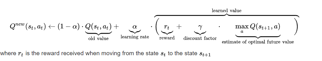
_{(source: https://en.wikipedia.org/wiki/Q-learning)}

Q-Learning is a reinforcement learning algorithm, which in its most simplified form, uses a table to store all Q-Values of all possible state-action pairs possible.

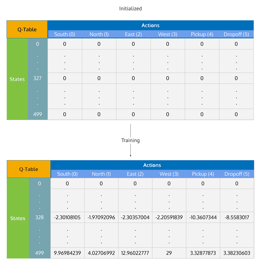
                                                                                                             _{(source: https://en.wikipedia.org/wiki/Q-learning)}

It updates this table using the formula mentioned above, while action selection is usually made with an ε-greedy policy.

A greedy policy essentially means that the agent is constantly performing the action that is believed to yield the highest expected reward. As such, this policy will not allow the agent any flexibility when it comes to exploring its environment. In order to fix this and allow the agent to explore, an ε-greedy policy is often used instead: a number (named ε) in the range of [0,1] is selected, and prior selecting an action, a random number in the range of [0,1] is selected. If that number is larger than ε, the greedy action is selected — but if it’s lower, a random action is selected.

How does Q Learning scale? What will happen when the number of states and actions become very large?

This is actually not that rare as even a simple game such as Tic Tac Toe can have hundreds of different states.

Enter Deep Learning! The combination of Q Learning and Deep Learning yields Deep Q Networks. This variant replaces the state-action table with a neural network in order to cope with large-scale tasks, where the number of possible state-action pairs can be enormous.

The main difference between deep and reinforcement learning is that while the deep learning method learns from a training set and then applies what it learned to a new dataset, deep reinforcement learning learns in a dynamic way by adjusting the actions continuous feedback in order to optimize the reward.

A good way to understand reinforcement learning is to consider a few practical examples and possible applications:

• Playing the board game Go.

The most successful example is mentioned AlphaGo, the first computer program to defeat a world champion in the ancient Chinese game of Go. Others include Chess, Backgammon, etc. AlphaGo uses reinforcement learning to learn about its next move based on current board position.

• Computer games.

Most recently, playing Dota 2, Doom, Atari Games.

• Robot control

Robots can learn to walk, run, dance, drive, fly, play ping pong or stack boxes/legos with reinforcement learning.

• Recommendation Systems

Microsoft has just introduced a new decision suite in its Azure cognitive services which features a reinforcement learning service for recommendations or personalization designed to improve user engagement.

• Online advertising.

A computer program can use reinforcement learning to select an ad to show to a user at the right time, or with the right format.

• Dialogue generation.

A conversational agent selects a sentence to reply based on a forward-looking, long-term reward. This makes the dialogue more engaging and longer lasting. For example, instead of saying, “I am 16” in response to the question, “How old are you?”, the program can say, “I am 16. Why are you asking?”

• Dynamic Pricing Models.

RL provides two main features to support fairness in dynamic pricing: on the one hand, RL is able to learn from recent experience, adapting the pricing policy to complex market environments; on the other hand, it provides a trade-off between short and long-term objectives, hence integrating fairness into the model’s core.

Conclusion:

Up to this point, this series has covered what a single neuron/perceptron is, how it processes information forward, how single neurons are grouped into layers to form an artificial neural network, the algorithms of gradient descent and backpropagation and briefly explained the supervised and unsupervised approach to learning.

This post adds on that knowledge base the concept of deep learning with an introduction to the reinforcement learning approach.

The next part of this series will cover in detail the more popular convolutional neural networks along with the versatile recurrent neural networks.

If you are a decision maker at your company, I hope this post and series has made you think and inquire how machine learning and RL can potentially be used to solve the business problems and challenges you’re facing.

If you are a researcher or if you’re just starting out, let’s connect and collaborate, there’s lots of areas to improve and potential research opportunities.

What are your thoughts? Can you think of any problem that RL could solve?

As always, the following resources will come in handy in acquiring a deeper and more practical understanding of reinforcement learning:

Reinforcement Learning: An Introduction — Richard S. Sutton and Andrew G. Barto

UC Berkeley Reinforcement Learning Course — http://rail.eecs.berkeley.edu/deeprlcourse/

Reinforcement Learning: State-of-the-Art (Adaptation, Learning, and Optimization) — Marco Wiering and Martijn van Otterlo

Hands-On Q-Learning with Python – Nazia Habib

I personally believe the best way to grasp new concepts is by trying to implement them yourself so if you’re looking for a more hands-on approach, try Andrej Karpathy’s Pong from Pixels project or the following repository that provides code, exercises and solutions for popular Reinforcement Learning algorithms: https://github.com/dennybritz/reinforcement-learning