Introduction to Deep Learning, Neural Network Basics

My main focus is Business Intelligence and Data Warehousing but recently I have been involved in the area of Machine Learning and more specifically Deep Learning to see if there are opportunities to use the technology from these fields to solve common BI problems.

Deep Learning uses interconnected networks of neurons called Neural Networks. These are loosely based on or perhaps it would be better to say inspired by networks of neurons in mammalian brains. For a more detailed definition see:- http://pages.cs.wisc.edu/~bolo/shipyard/neural/local.html

In recent years Neural Networks have been used to solve problems which conventional computer programs have struggled to do. They have been particularly successful in areas where problems are highly intuitive to humans but incredibly complex to describe, eg understanding speech or controlling a moving vehicle.

Let’s start then by looking at neurons and how they operate, they are after all the basic building block of a neural network. The simplest (and original) neuron is called the Perceptron, others which will be described here are the Sigmoid, Tanh and Rectified Linear Units (ReLu). This is not an exhaustive list but it’s a good place to start.

Perceptron

Below is a representation of a perceptron. It has 3 inputs (X₁, X₂, X₃) and one output, the inputs and the outputs are all binary values (0 or 1). It also has 3 Weights (W₁, W₂, W₃) and a Bias represented by “b”

The output of the perceptron can be 1 or 0. If the sum of the Inputs (X) multiplied by the Weights (W) is greater than the Bias then the Output will be 1, otherwise it will be 0.

Bias then is the threshold for the neuron to “fire” or in other words return an output of 1. If the bias is set to a high value then the neuron is resistant to firing, or it could be said to have a high threshold. It will need higher weighted inputs to fire. If the bias is set to a low number then the neuron has a low resistance to firing.

As an example then, consider the scenario where there are 3 inputs into the perceptron:-

W₁ has a weighting 0.7

W₂ has a weighting 0.4

W₃ has a weighting 0.2

Let’s assume then that for this example the bias is set at 0.8. Now lets work through some scenarios:

Scenario 1:-

X₁ has a value 0

X₂ has a value 1

X₃ has a value 1

Evaluating this scenario:

Input = SUM((X₁ * W₁) + (X₂ * W₂) + (X₃ * W₃))

Input = SUM((0*0.7) + (1*0.4) + (1*0.2))

Input = 0.6

As 0.6 does not exceed 0.8 the output of the Perceptron will be 0

Scenario 2:-

X₁ has a value 1

X₂ has a value 0

X₃ has a value 1

Evaluating this scenario:

Input = SUM((X₁ * W₁) + (X₂ * W₂) + (X₃ * W₃))

Input = SUM((1*0.7) + (0*0.4) + (1*0.2))

Input = 0.9

As 0.9 does exceed 0.8 the output of the Perceptron will be 1

This behaviour can be plotted as shown below, when the sum of the inputs multiplied by the weights exceed the bias (here 8) the output is 1 but less than the bias the output is zero:-

Other Neurons

The neurons below all behave in a similar way to the Perceptron, all can have multiple inputs and all have a single output. The output is always dependent on the inputs, weights and bias of the neuron. How they differ is in their their activation function, ie how they respond to the inputs.

Sigmoid

The Sigmoid Neuron has decimal inputs and outputs which are numbers between 0 and 1. The shape of the activation function is smoother than the stepwise shape of the perceptron, as shown below.

Explaining this in a little more detail, when the sum of the Weights multiplied by the Inputs is much lower than the bias the output is close to zero. As the bias is approached the output begins to rise until it is 0.5 at the point of the bias (still here the value of 8) after which as the weights and inputs sum increases it continues upwards towards the value one. This subtle difference provides Sigmoid neurons a significant advantage over Perceptrons as networks of Sigmoids are more stable in gradient-based learning, I’ll explain this in another blog later.

Tanh

The Tanh neuron is similar to the Sigmoid neuron except its rescaled to have outputs in the range from -1 to 1

Choosing between Sigmoid and a Tanh is sometimes a matter of trial and error, however it is sometimes said that Tanh learn better as Sigmoids suffer from saturation more easily, again I would have to expand the scope of this blog quite a lot to explain this though.

ReLu

The ReLu neuron (short for Rectified Linear Unit) returns 0 until the Bias is reached then increase in a linear fashion as shown below.

ReLu neurons are favoured over Sigmoid neurons in feed forward neural networks (see below) because they are less susceptible to a problem known as Learning Slowdown.

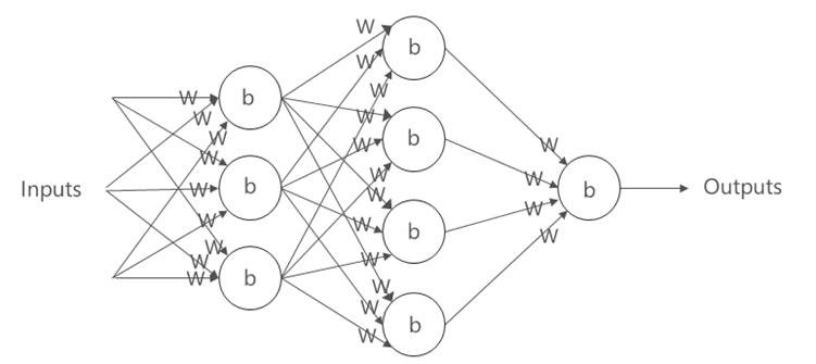
A Simple Feed Forward Network

Neurons can be linked together in different ways, the simplest design to explain is the Feed Forward Network. In the diagram below there are 3 layers of neurons with every neuron in a layer connected to every neuron in the next layer. Every neuron has an individual bias setting and every connection has an individual weight.

This is called a feed forward network because the flow from inputs to outputs is unidirectional, there are no feedback loops here and the network is stateless as the output is calculated from the input without effecting the network.

The network is trained by adjusting the Weights and Biases on each neuron until the desired output is are produced for the provided inputs. This training is usually done working from the outputs to the inputs with a method called Back Propagation. Back Propagation is a whole subject which can be explored more here:- https://pdfs.semanticscholar.org/4d3f/050801bd76ef10855ce115c31b301a83b405.pdf

There are 3 layers in a feed forward neural network, the input layer, the output layer and the layer in the middle which is called the hidden layer and which may itself be made up of several layers of neurons. In the diagram below the hidden layer has 3 layers of neurons. A neural network is considered “deep” if there are 2 or more hidden layers in the network.

In summary then this blog introduces a simple neural network and explains a little of how neurons work. There are quite a few more concepts which need to be introduced to get a full picture but hopefully you found this interesting and informative and I’ll try to fill in some of the gaps in future blogs.