Introduction

The first part of this series outlined how a perceptron processes information forward for an OR logic gate, however the parameters have been initialised to the exact values needed for such a gate and therefore there was no actual learning taking place.

This post explores the algorithms of gradient descent and back-propagation in order to understand the difference between them and their role in the learning process for artificial neural networks.

The next part of this series will cover in detail the concepts of deep learning and reinforcement learning.

Though you might find a number of explanations and tutorials for ANNs, different people have varied angles of seeing and understanding things as well as a personal unique emphasis of study.

You’ll still need to brush up on your algebra, calculus and probabilities if you want to dive deeper. There’s recommendations and links at the end of the post.

This series differs from the pile of maths, coding and calculation tutorials in its aim to explore ANNs from a different perspective which might in some sense enhance our understanding, so let’s dive in.

How do artificial neural networks learn?

The learning process for ANNs essentially means adjusting the parameters in order to reduce the difference between target output t, on each training case/iteration, and the actual output y, produced by the model. In other words, learning is a type of error correction and it will only occur when an error has been made, otherwise the parameters are left unchanged.

During training, it’s necessary to measure the performance of the network as it attempts to find the optimal parameters set. An error measure is used to find out how far the most optimal parameters are is the sum-squared error which is computed over all the input vector and output vector pairs in the training set. SSE is a commonly used measure but there are many other measures of error.

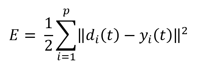
d(t) = desired output

y(t) = actual output

p = Number of input/output vector pairs in the training set.

Finding the right parameters for the network is done using gradient descent, which has two steps: calculating gradients of the loss/error function, then updating existing parameters in response to the gradients, which is how the descent is done. This cycle is repeated until reaching the minima of the loss function.

Gradient Descent

Gradient descent is an optimization algorithm used to minimize the loss function by iteratively moving in the direction of steepest descent as defined by the negative of the gradient.

Keep in mind that, the loss function is used to monitor the error in the output of a machine learning model. Minimizing any function means finding the deepest valley in that function or getting to the lowest error value possible. In short, the accuracy of the model is increased by iterating over a training data set while tweaking the parameters (the weights and biases) of the model.

By analogy, gradient descent method can be compared with a ball rolling down from a hill: the ball will roll down and finally stop at the valley.

Gradient descent steps:

1. Find the slope of the objective function with respect to each parameter/feature:
2. Pick a random initial value for the parameters.
3. Differentiate “y” with respect to “x”
4. Update the gradient function by plugging in the parameter values.
5. Calculate the step sizes for each feature: step size = gradient * learning rate.
6. Calculate the new parameters: new params = old params -step size
7. Repeat steps 3 to 5 until gradient is almost 0.

Learning rate is the size of the step, dictates how quickly the network converges. It is set by a matter of experimentation (usually small – e.g. 0.1) and tells how far to move the weights.

The smaller the rate the longer it will take to reach the minima, and the larger the rate the higher the risk of skipping the minima.

Think of a simple function that has one number as input and one number as an output.   The goal will be to start the input point and figure out in which direction to move in order to make the output lower.

The slope of the function where the input point is can be calculated and the point will move to the right if the slope is negative or move to the left if the slope is positive.

The aim is to iterate this in order to find the global minimum, notice that when the point approaches the minimum the number of steps increase. This helps the point from overshooting.

There are some optimisers that help avoid getting stuck in a local minima by following their own pattern and acting on either the learning rate or the gradient.

The following is a list of some of the most popular optimisers by the year in which the papers were published.

• Momentum – 1964 – Instead of depending only on the current gradient to update the weight, gradient descent with momentum replaces the current gradient with V (which stands for velocity), the exponential moving average of current and past gradients.
• AdaGrad -2011– Divides the learning rate by the square root of S, which is the cumulative sum of current and past squared gradients.
• RMSprop -2012– Instead of taking cumulative sum of squared gradients like in AdaGrad, it takes the exponential moving average of these gradients.
• AdaDelta -2012– Adadelta removes the use of the learning rate parameter completely by replacing it with D, the exponential moving average of squared deltas.
• Nesterov -2013– Similar to momentun this also utilises V, the exponential moving average of projected gradients.
• Adam -2013– Acts upon the gradient component by using V, the exponential moving average of gradients and the learning rate component by dividing the learning rate α by square root of S, the exponential moving average of squared gradients.

There are also variations of gradient descent, the three main types are:

1. Batch Gradient Descent: This type of gradient descent processes all the training data in a single step. However, if the number of training examples is large it can become computationally very expensive.
2. Stochastic Gradient Descent: This type of gradient descent processes one training example per iteration. The parameters are being updated after every single iteration in which only a single example has been processed. Hence, this is quite faster than batch gradient descent. But again, when the number of training examples is large the number of iterations will also large.
3. Mini Batch gradient descent: This type of gradient descent is faster than both batch gradient descent and stochastic gradient descent. It shuffles and splits the training dataset into small batches. The parameters are updated after each batch and it works for larger training examples.

 

Backpropagation

In machine learning, gradient descent and backpropagation often appear at the same time, and sometimes they can replace each other. Backpropagation can be considered as a subset of gradient descent, which is the implementation of gradient descent in multi-layer neural networks.

Backpropagation, also named the Generalized Delta Rule, is an algorithm used in the training of ANNs for supervised learning. (generalizations exist for other artificial neural networks) It efficiently computes the gradient of the error function with respect to the weights of the network for a single input-output example. This makes it feasible to use gradient methods for training multi-layer networks, updating the weights to minimize loss.

Since the same training rule is applied recursively for each layer of the neural network, we can calculate the contribution of each weight to the total error inversely from the output layer to the input layer.

Simply put, we’re propagating the total error backward through the connections in the network layer by layer, calculate the contribution (gradient) of each weight and bias to the total error in every layer, then use gradient descent algorithm to optimize the weights and biases, and eventually minimize the total error of the neural network.

The backpropagation algorithm has two phases:

Forward pass phase: feed-forward propagation of input pattern signals through the network, from inputs towards the network outputs

Backward pass phase: computes ‘error signal’ – propagation of error (difference between actual and desired output values) backwards through network, starting form output units towards the input units.

Visualising this can help understand how the backpropagation algorithm works step by step

 

 

 

Now that we have a better understanding of a ANN learns let’s have a look at the two main types of learning; Supervised and Unsupervised.

Supervised Learning

In the supervised learning approach, the training data consists of a set of labelled examples and an algorithm such as ANNs can be used to learn the mapping function from the input to the output.

The goal is to approximate the mapping function so well that when new input data (x) is given it can predict the output variables (Y) for that data.

The name of supervised learning comes from the learning process of the algorithm that learns from the labelled data very similar to how a pupil learns with the guidance of a teacher. The correct answers are known, so the algorithm iteratively makes predictions on the training data and is corrected by the “teacher”. Learning stops when the algorithm achieves an acceptable level of performance and it is then tested on new data to determine its accuracy.

A downside of this approach is that labelled data can be difficult and expensive to acquire as it still takes people to manually go over the data and label it.

There are two main types of supervised learning:

• Classification: A classification problem is when the output variable is a category/class and the goal is to classify the input into the known categories/classes. It basically aims to predict which class the input corresponds to. Some examples include systems where we seek a yes-or-no prediction, such as “Is this tumour cancerous?”, “Does this product meet our quality standards?”
• Regression: A regression problem is when the output variable is a real and continuous value. Here, the goal is to predict the output value given an input x. Some examples include systems where the value being predicted falls somewhere on a continuous spectrum like predicting the stock price of a company or predicting the temperature tomorrow based on historical data.

Some popular examples of supervised machine learning algorithms are:

• Artificial Neural Networks.
• Linear & logistic regression.
• Decision tree & random forest.
• Support vector machines.
• Naïve Bayes

Unsupervised Learning

In the unsupervised learning approach, there is no labelled data, an algorithm is used to model the underlying structure or distribution in the data in order to discover the patterns and learn more about the data.

It is called unsupervised learning because unlike supervised learning approach there is no correct answers and there is no teacher to correct the algorithm.

As there are no training examples used in this process, the algorithm is given a dataset and is then tasked with finding the patterns and correlations within. One example would be identifying close-knit groups of people in social network data.

There are two main types of unsupervised learning:

• Clustering: Here the goal is to find similarities in the dataset and group similar data points together. Cluster analysis can be used for market segmentation where a customer dataset is divided into different market segments for each customer type. This method can also be used to detect anomalies that do not fit to any group.
• Association: Here the aim is to discover rules that describe large portions of our data, such as people that buy X also tend to buy Y. A classic example of association rules would be market basket analysis, like, a person who buys potatoes and burgers usually buys beer too.

Some popular examples of unsupervised learning algorithms are:

• Artificial Neural Networks
• K-means clustering
• K-NN (k nearest neighbours)
• Apriori algorithm

The data volume, structure and problem being solved will usually dictate on whether to use supervised or unsupervised learning.

So far, this series has shown what a single neuron/perceptron is, how it processes information, how single neurons are grouped into layers to form an ANN, the algorithms used by an ANN to learn and briefly explained the supervised and unsupervised approach to learning.

With the intuitive understanding we’ve built so far in the next part of this series we will explore the concept of deep learning and dive into the details of the third type of learning, reinforcement learning.

As always, if you’re keen on understanding what has been covered so far in more detail, the following resources will come in handy;

• Machine Learning: An Algorithmic Perspective – Stephen Marsland
• The Elements of Statistical Learning: Data Mining, Inference, and Prediction – Trevor Hastie, Robert Tibshirani, Jerome Friedman
• Neural Networks and Deep Learning – Michael Nielsen (chapter two covers backpropagation theory, architectures, and applications)

Want to know more about data science?

Dan Fitton provides a great overview of what data science is.

https://adatis.co.uk/data-science-what-it-is-and-why-it-matters/

What is and how to prevent over fitting?

Tom Jordan explains it in detail:

https://adatis.co.uk/4-ways-to-prevent-overfitting-in-machine-learning/

Machine Learning Interpretability:

https://adatis.co.uk/ml-interpretability-what-it-is-and-how-it-affects-us/

AI in retail: How predictive analytics drive smarter strategic decisions:

https://adatis.co.uk/ai-in-retail-how-predictive-analytics-drive-smarter-strategic-decisions/

Sentiment Analysis in Power BI:

https://adatis.co.uk/integrating-cognitive-services-text-analytics-within-powerbi-part-1/