Introduction to Artificial Neural Networks

Introduction

This blog post is the first of a 5-part series which aims to demystify and explain what artificial neural networks (ANN) are and how they learn. It will also showcase a few commercial examples where they have been successfully implemented.

As the series is aimed at both technical and non-technical people, the first parts of the series will focus on gaining a conceptual understanding and as we progress the last posts will emphasise more on the mathematics, coding and tools.

It’s not difficult to understand the idea of ANN on a conceptual level and once you learn what they are and understand how they work the math and code will be more intuitive.

Implementing them is a challenge because of hardware or cloud dependence as well as the fact that they are purely “black box” models providing very little insight into what these models really do.

For anyone interested into a deeper dive in the maths behind neural networks there are books that cover it better and are much more in depth than a blog post can do it justice. There will be recommendations to resources at the end of the post.

For this first blog, we’ll start by understanding what a single neuron is, what are its components and how it processes data followed by an overview of how neurons are grouped together in layers in order to form a neural network.

In the second part we’ll dive into the different types of learning and explain how a network learns using the algorithms of gradient descent and back-propagation along with a couple of their variations.

The third blog will cover the two methods of deep and reinforcement learning while outlining the difference between the two and exemplifying them with specific commercial use cases.

The 4th post will be showcasing the more popular convolutional neural networks, recurrent neural networks and the hot and trendy generative adversarial neural networks.

The final post will focus on how to code a GAN neural network using Azure Notebooks, Python and the Keras library which will run on top of Microsoft Cognitive Toolkit.

What is a neuron?

It’s estimated that the human brain contains around 86 billion neurons, each connected to about 100,000 of its immediate neighbours thus creating complex networks that helps coordinate all the necessary functions of life.

A biological neuron, also known as a nerve cell, is a cell that takes in, processes and transmits information through electrical and chemical signals. It is one of the basic elements of our nervous system.

The artificial neuron is modelled based on the biological one and can be represented as a mathematical function or a single processing unit that is part of a network. As with the biological neuron the artificial one is also connected to other neurons in the network.

The first artificial neuron which was called the Perceptron and was invented in 1958 at the Cornell Aeronautical Laboratory by Frank Rosenblatt, funded by the United States Office of Naval Research.

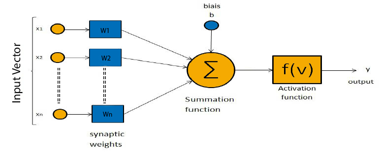
From the diagram above we can see that a single neuron has 6 components :

1. Input Vector
2. Synaptic Weights
3. Bias b (threshold = -b)
4. Summation function ∑
5. Activation function f(v)
6. Output y

The connections between an individual neuron represent the inputs and outputs of the neuron. The neuron will assign a specific weight to each of its connections, the weight is used to indicate the importance of a specific input – the higher a weight, the stronger an input is.

Each neuron also has a bias(b) term which is added to individual weight/connection and allows us to shift the activation function by adding a constant to the input. This can be thought of as the similar role of a constant in a linear function in which the line is effectively transposed by the constant value.

Every time an input vector x is passed through, the neuron will calculate the weighted average of the values of the vector x, based on its current weight vector w and adds the bias.

output = sum (weights * inputs) + bias

Lastly, the result from this calculation will be passed through a non-linear activation function.

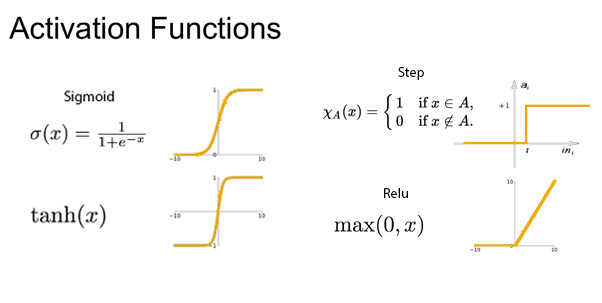
There are many types of functions that we can use as activation functions for neurons depending on the output we prefer.

For example, the step activation function is quite easy to understand, if the weighted sum of the inputs is bigger than 0, the neuron will signal a 1, otherwise a 0. However it’s not always the case of signalling a 1 or 0 as an artificial neuron can output any positive or negative number depending on the kind of activation function that is in use.

To better understand let’s see how a perceptron can implement an OR logic gate.

For the example above, the weights and bias have been initialised to the exact value needed for an OR logic gate implementation. But how does a perceptron adjust its weights and bias when they have been randomly initialised?

We’ll take an in depth look at the algorithms used by perceptron to learn in the next blog post.

Now that we have a solid understanding of how a perceptron processes information forward let’s group multiple perceptron’s together to form a neural network.

What is a neural network?

From the diagram above we can see how each individual neuron is connected to the other neurons in the previous and next layer thus forming a network that allows communication between the individual neurons. The inputs from one layer of neurons are received and processed, as exemplified with the perceptron, in order to generate an output which is then passed to the neurons in next layer of the network.

It is important to note that each individual neuron operates only locally on the inputs it receives via its connections.

The first layer in a neural network is most often named as the ‘’input layer’’ as it’s the layer that accepts the initial data inputs while the last layer is named the ‘’output layer’’ as it’s the layer that produces the final output. All the other layers between the input and output layer are named the hidden layers.

It is through the connections between the neurons and their respective weights which are adjusted based on the presented data that a neural network is able to train and learn.

In other words, ANNs “learn” from examples and exhibit some generalization capability beyond the training data.

A couple of questions to consider when thinking about an artificial neural network.

How do we set the initial values of the weights?

There are different techniques depending on the type of network it is and the problem you’re trying to solve but the most popular/optimal way is to randomly distribute the weights between -1 and 1 as it helps prevent a bias towards any particular output.

How many neurons per layer?

This depends on which layer, for example, the input layer will always have the same number of neurons as the number of features (columns) in your data.

The output layer’s number of neurons will always depend on what type of network it is, if it’s a classifier type of network it will have the same number of neurons as the class labels we want to be outputted and if it’s a regressor type of network it will have one neuron that outputs a single value.

For the hidden layer there are some empirically-derived rules-of-thumb, the most popular of these:

• The number of hidden neurons should be between the size of the input layer and the size of the output layer.
• The number of hidden neurons should be 2/3 the size of the input layer, plus the size of the output layer.
• The number of hidden neurons should be less than twice the size of the input layer.

These three rules can be used independently and are only a starting point for us to consider when thinking of the problem and architecture of the network but ultimately the selection of an architecture for a neural network will come down to trial and error.

How many layers in a network?

There isn’t a specific number for how many layers a neural network should have as it’s dependable on the problem we are trying to solve. If it’s a linear separable problem then the network doesn’t need any hidden layers while one or more hidden layers can approximate any function and can learn to draw shapes around examples in a high-dimensional space that can separate and classify them, overcoming the limitation of linear separability.

How do we train a neural network?

There are two main types of training a neural network.

• Sequential mode (on-line or per-pattern) – weights are updated after each pattern is presented.
• Batch mode (off-line or per epoch) – weights are updated after all or a batch of patterns are presented

Summary

So far, we’ve seen what a single artificial neuron is and how it processes information forward as well as how grouping single neurons into layers form a network.

There was no efficient algorithm for training multi-layer neural networks until Rumelhart and McClelland proposed the backpropagation algorithm in 1986, in the next part of this series, we’ll take a look and understand how a neural network calculates its error and how it is able to actually learn using gradient descent and backpropagation.

If you’re interested in knowing more about the history and a more comprehensive view of the perceptron I would recommend the classic “Perceptrons: an introduction to computational geometry” written by Marvin Minsky and Seymour Papert or if you’re just too excited and want to know more about ANN I would also recommend checking out “Make Your Own Neural Network” by Tariq Rashid.

One last recommendation is the “Deep Learning” book written by Ian Goodfellow, Yoshua Bengio and Aaron Courville, it’s intended to help students and practitioners enter the field of machine learning in general and deep learning in particular.