
You have watched all the machine learning videos on YouTube, and you have completed every Python tutorial Code Academy can throw at you. You already have an eye on your first Kaggle competition to make your first steps towards data science stardom, your name revered within niche Facebook groups alongside Andrew Ng and Geoffrey Hinton. You settle down to train a simple classifier on the Iris dataset and have 99% and above accuracy on the dataset. Great!
It’s then time try out some other data points that your model hasn’t seen before – and it doesn’t quite perform as expected. New data point after new data point predicted incorrectly, even when the values are only slightly different from the data that the model was trained on. The future glory, the published research and the Nobel Prizes have suddenly faded away, and you feel you have fallen at the first hurdle.
But before falling into inconsolable despair, there is no need to worry, as this is a well-researched and well-documented phenomenon within data science. In this blog we will be learning about said effect, overfitting, and then exploring some of the most frequently used techniques in machine learning to prevent it.
What is Overfitting?
The definition of overfitting is given by the Oxford Dictionary as:
The production of an analysis which corresponds too closely or exactly to a particular set of data, and may therefore fail to fit additional data or predict future observations reliably.
In the context of machine learning, it is when the model has become incredibly specialised towards the data that it has been trained on, gaining the ability to predict even anomalous points within this set of data. However, the model now will not be able to follow the general pattern for prediction from the field you wish to apply it to.
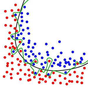
Figure 1 is a great example of this effect, where the green line shows the boundary for prediction between red and blue for the overfitted model while the black line shows the boundary for an optimal model. While the optimal model boundary may create some errors in prediction, it follows the general trend shown by the data set to a greater degree to the overfitted model. The ability to follow the general trend is the generalisability of a model.
Now that we understand the theory behind overfitting, we can begin looking at ways to prevent it…
Validation Sets and Early Stopping
This first technique used requires the data set to be broken down into three sub sets, the training, validation and test set. The training set contains the data that is used to train the model (as expected), while the validation and test sets contain data that is unseen to the model that is used to evaluate its effectiveness. Evaluation on the validation set takes place at regular intervals during the training process, while a test set evaluation typically takes places on the fully trained model, when wishing to compare accuracy of different models. A typical split of the dataset would be 80% for the training set, and 10% each for the validation and test sets.
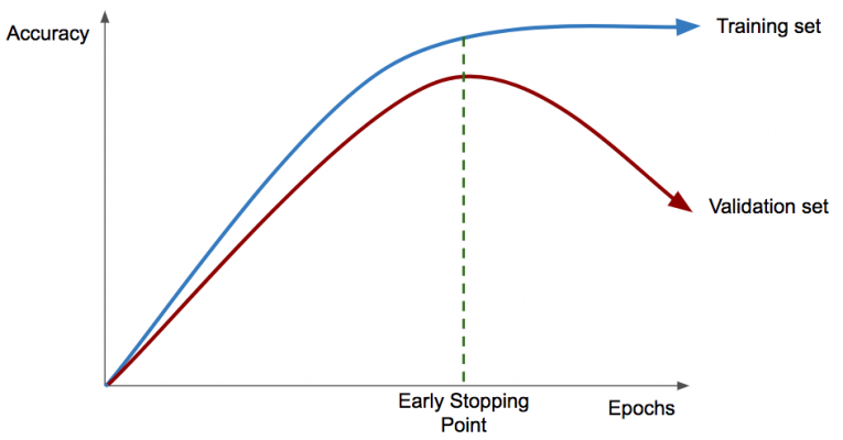
Early stopping is a simple, but effective, method to prevent overfitting. The effectiveness of the model is evaluated on the accuracy from the validation set, rather than the training set. When the validation accuracy begins flatlining, or even decreasing, the training process stops, with the model corresponding to the highest validation accuracy taken as the final model. This point is known as the early stopping point, and can be clearly seen in figure 2.
Removing Anomalies and Redundant Features
As we can see in figure 1, overfitting can be caused by the model taking account of anomalous points which break the general trend of the data set. A straightforward and easy to implement way to prevent the model taking account of these points in training is to simply remove them from the data set, where they then will not be able to influence the model. Obviously, this will not be applicable with all datasets, especially large and complex ones, but highlights the importance of knowing and understanding data before working with it.
A similar method for deterring overfitting is the removal of redundant features from your data set. These are columns which are irrelevant to making a predictive model from the training data, with data columns involving ID or serial numbers often being a great place to start, due to them being allocated sequentially. During the training process, any pattern existing in the training set with these redundant features can influence the model created, harming generalisability. An added benefit to removal of these irrelevant features is the reduction to training time created by the decrease in data.
L1 and L2 Regularisation
These two techniques, while being general statistical techniques and used within many machine learning processes, are frequently used in the training of neural networks, a sub class of machine learning models. These models are used within some of the most complex and intriguing research areas within artificial intelligence, such as Computer Vision and Natural Language Processing. Whilst more information on neural networks can be found here, it is enough to understand that they are formed of sub units called neurons, which each have several parameters associated with them.
Regularisation refers to the prevention of overfitting, and in this example is used within the loss function. This is a metric that is minimised during the training process in order to maximise accuracy. Neural networks that have been overfitted tend to have very large parameter values, as they adjust to all the anomalies in the data set rather than the general trend. By summing the value of all the parameters and adding this to the loss function, the minimisation of the new metric formed prevents large value parameters being formed, therefore preventing overfitting taking place.
The described process is for L1 regularisation, which can be extended into L2 regularisation by summing the squared value of the parameters and adding to the loss function. Both of these techniques have alternative names, being called Lasso and Ridge regularisation respectively.
Dropout
This technique is exclusively used within the training of neural networks, so isn’t applicable to all machine learning models, however can be used in the production of extremely effective neural network models. During the start of each step in the training process, each sub unit of the model, the neuron, has a probability of being included in that step or not. If it doesn’t make the cut, it is effectively deleted from the network for that step, and then reintroduced on the next step.
This may seem incredibly counterintuitive, as it effectively limits the amount of time the whole model has in training. However, dropout limits the exposure of each neuron to anomalies within the dataset, improving the generalisability of the model. Do not worry if this technique is confusing or hard to follow, it mainly exists to illustrate some of the quirks in the training of neural networks!
Conclusion
Within this blog post, we have learned about some common methods for preventing overfitting within machine learning, from very simple to more complex examples, however have hardly scratched the surface of the wild world of improving generalisability. There are many more methods that could be used, such as DropConnect and k-Fold Cross Validation, and currently there is active research going into wilder and wackier methods of regularisation.
Finally, I hope this blog post has provided some insight into the training of machine learning models, a task which can be both highly challenging and extremely rewarding, and some advice into its implementation. I can’t promise to have fulfilled your dream of implementing SkyNet, but hopefully this has taken you a step closer!


Thanks