Top 10 Power BI Performance Tips (Part 2)

In Part 1 of this four part-part blog series we identified and explained the first 5 performance tips that should be incorporated during your Power BI development process. If you haven’t read it, be sure to check it out, especially as it highlights the most important performance tip. Now, let’s continue with the next 5 performance tips which should be incorporated to further improve the performance of our Power BI solutions.

This blog series will highlight the top 10 tips for performance and best-practice. Each blog will be broken down into the following parts:

• Top 10 Power BI Performance Tips (Part 1)
• Top 10 Power BI Performance Tips (Part 2)
• Top 10 Power BI Best-Practice Tips (Part 3)
• Top 10 Power BI Best-Practice Tips (Part 4)

Tip 5) Question Calculated Columns

When we need to create some form of calculation in addition to the data we already have in our model, we have the option to use a Calculated Column or a Measure. I have worked with many individuals in optimising their Power BI solutions and I find that calculated columns are highly used in comparison to measures, as they seem to be the preferred option when constructing a calculation through a DAX formula. From all the discussions I have had, many times this simply comes down to the physical presence that calculated columns have in the model and due to calculated columns feeling more like home, meaning more similar to Excel. This was especially the case when I was working closely with individuals with a financial background and were big in using excel.

What is a Calculated Column?

A Calculated Column is processed at the point of refresh and is stored inside the database. Therefore, if you go to the ‘Data’ tab you will see the physical column added to an existing table in your model. As calculated columns are physically stored in the database, this means they consume disk and more importantly valuable memory which we should always look to preserve and use efficiently. Furthermore, calculated columns operate on Row Context, which is a type of evaluation context that works on an iterating mechanism which starts on the first row of the table the calculated column has been placed in and evaluates the expression for each and every row until it reaches the last row.

What is a measure?

A Measure is processed at the point of interaction, therefore when the measure is added to a visual on the Power BI canvas. This means it is not stored in the database, therefore does not consume memory as the calculated column does. However, as measures are processed at the point of interaction, they will be consuming CPU instead. Also, measures use another type of evaluation context, which is Filter Context. This type of evaluation context refers to the filtering that is applied to the tables in the underlying model which in effect influences the result of a measure.

We have mentioned the different types of Evaluation Context that exist for calculated columns and measures. It is very important to understand the concept of Evaluation Context in order to have a good understanding on writing DAX and the behavior of measures vs calculated columns. I have previously posted an article on Evaluation Context: Understanding DAX through the Power of Evaluation Context.

The reason we should question the use of calculated columns over measures is due to the combination of two things.

Firstly, calculated columns are almost the default choice when the need to add additional data to the model arises. Secondly, calculated columns consume memory due to physically being stored in the database. Therefore, we end up with Power BI solutions that have tens or hundreds of calculated columns which are consuming memory. This is the core reason for questioning whether a calculated column should be used. Can we use a measure instead? Doing this will reduce memory consumption, improve refresh times and enable publishing Power BI solutions to the service that were previously exceeding the 1GB limit (Pro licensing).

Tip 6) Disable Auto Date/Time

You may not know but for every date column ingested or derived in Power Query and loaded to the Power BI model, a date table is auto-generated in the background. Now, it’s quite understandable that many are not aware of this, after all, these tables are not visible through the Power BI Desktop. The reason for these auto-generated date tables being produced is to support time-intelligent functions in reporting and to offer the capability of aggregating, filtering and drilling-through the date attributes Year, Quarter, Month and Day.

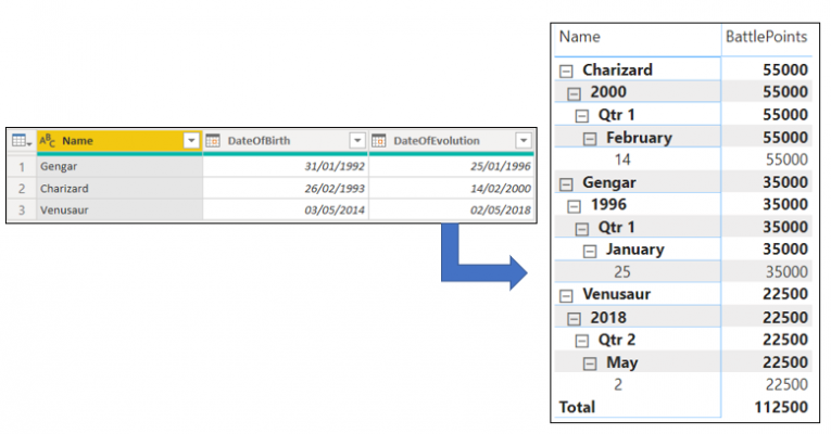
When these tables are generated by Power BI a relationship is established between the date column in the auto-generated table and the date column from the initial table in the model. However, these again are not visible from Power BI Desktop. Furthermore, these date tables can hold a high number of records due to holding all possible date values between the minimum and maximum date. For instance, in the table above we have the column ‘DateOfEvolution’ which holds the minimum date 25/01/1996 and the maximum date 02/05/2018, meaning we will have 8,133 rows which are all the dates between the minimum and maximum.

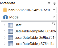
All these tables consume memory, therefore we should look to disable this feature. To identify these tables, we can either use the VertiPaq Analyzer or DAXStudio. By using DaxStudio to establish a connection to our Power BI model we will have a view of the auto-generated tables that have a prefix of “LocalDateTable_”:

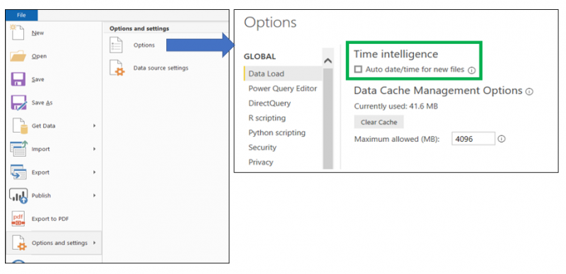
Imagine having a very large model and every table in the model consisting of data columns, with every data column having a wide range between the minimum and maximum date. This will increase memory consumption. Disabling this feature in the past was very frustrating as it was required to be done for every Power BI Desktop that was launched. However, since May 2019 (I think) disabling auto-generated date tables has been added to the Global Settings, meaning once disabled it is applied moving forward to any future Power BI solutions launched. To disable this feature, in Power BI Desktop click on File, select Options and settings, Options and under the Global settings select Data Load and deselect the Auto date/time option as the below illustrates:

Tip 7) Disable Data Preview downloading in Background

When we use Power Query, the top 1000 rows are stored in memory which in return displays a preview of the data. When working with a large model that consists of multiple queries in Power Query, this can raise some performance issues.

In the past, I was working on a Power BI solution with multiple queries which was continuously lagging on the ‘Evaluating’ status against all queries when triggering a full model refresh. This resulted in forcing Power BI desktop to close due to none of the queries moving to a ‘Loading Query’ status, therefore being in an unresponsive state. This is when I started to experiment with the option ‘Allow data preview to download in background’ which once disabled, dramatically increased performance as all the queries that were previously stuck in the ‘Evaluating’ status started loading successfully with no delay on a full refresh. From my understanding, the reason this was occurring is due to a full model refresh not only triggering the query load, but also the data preview to be loaded in the background, therefore consuming further resources. Chris Webb has a great article on this which I would recommend.

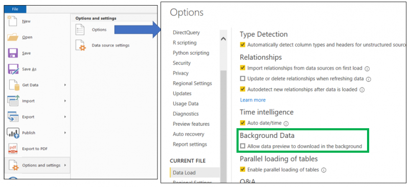
To prevent these previews from being downloaded, we can deselect the feature ‘Allow data preview to download in the background’ directly in Power BI Desktop by clicking on File, Options and settings, Options and Current File, as the below image illustrates:

Tip 8) Integers before Strings

After ingesting data into Power BI by selecting the required data connector and connectivity type, you then have the option to apply transformations and shape the data to the required format using Power Query. The next step is processing the data, therefore loading the data to Power Pivot, which is an in-memory columnar database for storing your model and works of the compression engine VertiPaq. The VertiPaq engine, also known as xVelocity, conducts three types of compression for reducing the overall memory consumption: Value Encoding, Dictionary (Hash) Encoding and Row Level Encoding (RLE).

Now, understanding these various types of compression in detail is out of scope for this blog, so to understand them more I would highly recommend reading ‘The Definitive Guide to DAX’, which offers a wealth of valuable information on VertiPaq. With that said, we will be highlighting two of these, as they are key to understanding why we should aim to use integers over strings in Power BI.

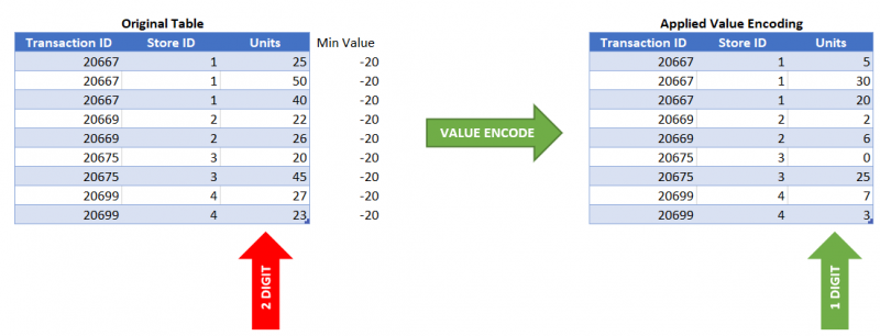
Value Encoding

This is whereby a column is reduced in memory through the VertiPaq engine identifying the minimum value in the column and subtracting all the other values by this minimum value. For example, in the below image we can see the minimum value in the column Units is 20, therefore the first row of 25 Units will become 5 Units (25-20), the second row of 50 Units will become 30 Units (50 -30), the third row of 40 Units will become 20 Units (40-20) and so on. Therefore, it is reducing the number of digits, meaning the number of bits consumed. During query time, in order to retrieve the correct number of Units the VertiPaq engine simply adds the minimum back to the number originally subtracted. A very important note, as obvious as it may be, is that Value Encoding only works with integer values. This is important to remember.

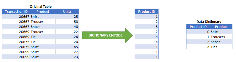
Dictionary Encoding

This is whereby a column with string values is reduced in memory through the VertiPaq Engine creating a data dictionary table which consists of two columns:

• A distinct ID column for uniquely identifying each string value
• A column containing the string value

Once the data dictionary table is created, the distinct ID’s from the data dictionary are referenced to the values in the original column. If you have ever used the VertiPaq Analyser for optimising your solution, you would have seen something called ‘Dictionary Size’, which is exactly this. An important note is understanding that the higher cardinality in the column, the larger the memory consumption from the data dictionary.

So here it is, after highlighting the above, we should aim to use integers over string values as we would be promoting Value Encoding which does not create a Data Dictionary table which consumes more space.

Tip 9) Use Query Reduction (Slicers, Filters & Cross Highlighting)

With all the previous performance tips, they were more based around the use of Import as a connectivity type, therefore the in-memory mode, whilst this performance tip will focus more on DirectQuery. If you are using DirectQuery and you have optimised the underlying database as much as possible and still need that extra bit of performance, it might be worth trying this out.

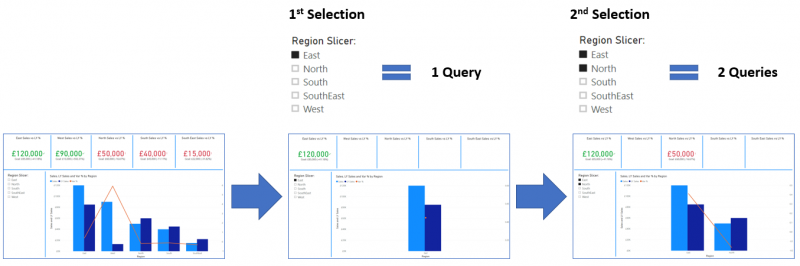
With DirectQuery, a query is generated and sent to the database at the point the report consumer interacts with the report by selecting a value in the slicer, selecting one of the bars in the column chart, using a filter or anything else. This can create a bottle neck, especially if you have a large number of users interacting with the Power BI report.

This is when Query Reduction comes into play, as it offers the capability to group various selections from Slicers and Filters into single queries, rather then generate a single query for every selection. For example, if I select the value ‘East’ from my Region Slicer a single query is instantly sent to the database and once I select the value ‘North’ a second query is sent to the database.

With Query Reduction, the query will only be sent to the underlying database once its confirmed by selecting the ‘Apply’ button as the below shows:

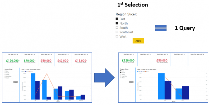
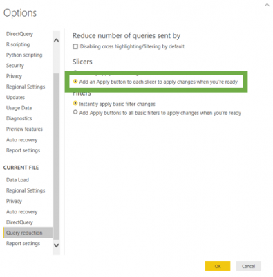
To apply Query Reduction for Slicers (or Filters), whilst in Power BI Desktop, select File, Options and settings, Options, Query Reduction and enable ‘Add an Apply button to each of slicer to apply changes when you’re read’, as the below illustrates:

Query Reduction doesn’t stop with Slicers and Filters, you can also select the box ‘Disable cross highlighting/filtering by default’. This prevents on-screen visuals acting as filters to other visuals, as again, selecting an element from a visual automatically filters other visuals, therefore, generates underlying queries to the database. If this is not needed, let’s go ahead and turn them off or at least reduce the amount of cross highlighting/filtering which is enabled by default.

Tip 10) Use Variables in your DAX

When we are writing DAX, we should always look to use variables instead of the measures themselves, as they improve readability and the process of debugging, reduce the complexity of the DAX and more relevant to this blog, have the capability to increase performance by stopping calculations from being re-calculated multiple times. So, by defining a calculation as part of a variable, once the calculation happens, the result is stored in the variable.

TY vs PY Var % =
DIVIDE (
    [TY Sales] - CALCULATE ( [TY Sales], SAMEPERIODLASTYEAR ( 'Retail 2'[Date] ) ),
    CALCULATE ( [TY Sales], SAMEPERIODLASTYEAR ( 'Retail 2'[Date] ) )
)

The above formula is a very common way in which I find the ‘Variance %’ calculated between an actual value and target value, which in this case is the Current Yearly Sales against the Previous Yearly Sales. As you can see from the above formula, the measure that calculates the Previous Yearly Sales is repeated twice, therefore it is re-calculated. This can be even more inefficient when working with iterator functions, but regardless in this case we can add the Previous Yearly Sales in a variable which returns the expected result but in less time. Reza Rad has a great article on DAX variables.

TY vs PY Var % =
VAR PreviousYearSales =
    CALCULATE ( [TY Sales], SAMEPERIODLASTYEAR ( 'Retail 2'[Date] ) )
RETURN
    DIVIDE ( [TY Sales] - PreviousYearSales, PreviousYearSales )

Summary

That’s all for my Top 10 Power BI Performance Tips. I hope you found these useful and start incorporating them throughout your Power BI development process, as they are sure to result in Power BI solutions that offer a higher quality experience to your organisations and report consumers. Also, I would highly recommend that you start using both the VertiPaq Analyzer for understanding the true memory consumption of the model in your underlying solutions and DAXStudio for understanding the performance of your DAX formulas. Stay tuned for Part 3, where we will start exploring the Top 10 Power BI Best-Practise Tips.