Loss Functions and Gradient Descent in Machine Learning

In an earlier blog I explained some of the basic building blocks of Neural Networks and Deep Learning (here). This was very high level and omitted a number of concepts which I wanted to explain but for clarity decided to leave until later. In this blog I will introduce Loss Functions and Gradient Descent, however there are still many more which need to be explained.

Loss Functions are used to calculate the error between the known correct output and the actual output generated by a model, Also often called Cost Functions

Gradient Descent is an iterative optimization method for finding the minimum of a function. On each iteration the parameters in a model are amended in the direction of the negative gradient of the output until the optimum parameters for the model are identified.

These are fundamental to understanding training models and are common to both supervised machine learning and deep learning.

An Example

A worked example is probably the easiest way to illustrate how a loss function and gradient descent are used together to train a simple model. The model is simple to allow the focus can be on the methods and not the model. Lets see how this works.

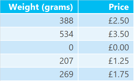
Imagine there are 5 observations of the weight vs cost of a commodity, The object is to train a model to allow it to be used to predict the price for any weight of the commodity.

The observations are:-

I plot on a graph the Weight vs the Price and observe the following

Modelling this as a linear problem, the equation of a line is of course

y = Wx + b

where W = slope of the line and b is the intersection of the line on the y axis.

To make the problem simpler please accept the assumption that b = 0, this is logically reasonable as the price for zero grams of a commodity is reasonably zero and this is supported by the data.

The method described here to train the model is to iteratively evaluate a model using a loss function and amend the parameters in a model to reduce the error in the model. So the next step is to have a guess at a value for W, if doesn’t need to be a good guess, in machine learning initial values are often randomly created so they are very unlikely to be anywhere near accurate on a first iteration. The first guess is shown in red below:

Now its necessary to evaluate how bad this model is, this is where the loss function comes in. The loss function used here is called Mean Squared Error (MSE). For each observed point the difference between the observed (actual) value and the estimated value is calculated (the error is represented by the green lines in the diagram below). The errors are squared and then the average of the squared observations is taken to create an numerical representation for the error.This error is plotted on a graph showing Error vs Slope (W) This Error graph will be used in the Gradient Descent part of the method.

Following this a small change to the value of W is made and the error is re-evaluated. In the graph below the original value for W is shown in blue the new value in red. The error is once again plotted on the error graph. The error graph reveals that the error is smaller and therefore the adjustment to the value of W was in the correct direction to reduce the error, in other words the model has been improved by the change.

Small increments are made to the value of W to cause a reduction in the size of the error, ie to reduce the value of the loss function. In other words we want to descent the gradient of the curve until we find a minimum value for the loss function.

Continuing the example, see below how we have continued to zoom in on a solution after several iterations.

At a certain point continued changes in the same direction cause the model to become worse rather than improve.

At this point the optimal value for W can be identified, its where the gradient of the error curve reaches zero or in other words the value of W pertaining to the lowest point on the graph (indicating the minimum error).

Summarising this then, the Loss function is used to evaluate the model on each training run and the output of the loss function is used on each iteration to identify the direction to adjust model parameters. The optimum parameters create the minimum error in the model.

Going forward we need to apply these 2 principals to explain Backpropagation, Backpropagation is the method by which Neural Networks learn, its the setting of all the Weights and Biases in the network to achieve the closest output possible to the desired output. That is for another blog which I hope to bring to you soon.