Meandering Through R (Part 1: Working with Data)

What is R?

R is an open-source programming language commonly used for statistics, machine learning and data analysis. It is no surprise that R is widely used in the data science and analytics community, as the creators of R were statisticians themselves. Building on top of S programming language, Ross Ihaka and Robert Gentleman designed R primarily for common data science and research tasks, such as importing data, data transformation, data manipulation, data exploration, statistical modelling, as well as data analytics and visualisation.

In this blog series, I am not arguing that R is better (or worse) than Python or any other language. In my opinion, an effective team should have a combination of language skills. My aim is to demonstrate some of the features of R to encourage a greater understanding.

Fundamentals

On the official website, R is referred to as an “environment within which statistical techniques are implemented”. This means that it aims to be a versatile and coherent system, instead of a bespoke and rigid data analysis software.

Here is how it looks:

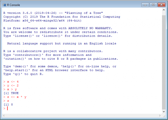
The first thing you probably notice is the use of <- as an assignment operator. Although the = can also be used, <- is preferred. This is mainly because <- is used solely for object/variable assignment. = on the other hand, can also be used in functions and case statements.

In terms of data types, R offers:

• Logical
• Integer
• Double
• Character
• Complex

A logical type is a Boolean, either TRUE or FALSE. Integers and doubles are both numeric data types, with integer being a whole number, and double a decimal. A character is a string and a complex is a rare type that includes real and imaginary parts, e.g. 2 + 0i.

As for data structures, the main ones are:

• Vectors
• Lists
• Matrices
• Data frames
• Factors

I am not going to go into detail about these here. That said, a vector is a single-dimensional sequence of data of the same data type, with indexing starting at 1; a list is an object that can contain different data structures and data types, in different sizes; a matrix is similar to a vector, but has two dimensions rather than one, arranged into rows and columns; a data frame is how datasets and tables are stored, with columns as variables; and a factor is for categorical variables. Note that 0-dimensional scalars do not exist. In R, they are vectors of length one.

When creating a classification or regression model, factors are quite powerful, eliminating the need for dummy variables or one-hot encoding. They also allow you to easily set the levels of categories if the data is ordinal, e.g. if you have a month column or a scale from strongly agree to strongly disagree.

Going Further

In programming, it is generally advised to comment code as much as possible. This helps with the readability and reproducibility of code. R is no different. You should be explaining what certain bits of code do and why you have made certain decisions by using comments. In R, comments are made by using the # prefix.

A handy feature in R is the use of the dollar sign ($) as a shorthand operator to access components of a data frame or list, i.e. table_name$column_name. When using an integrated development environment (IDE), this is especially convenient, as the full list of elements available is displayed when typing.

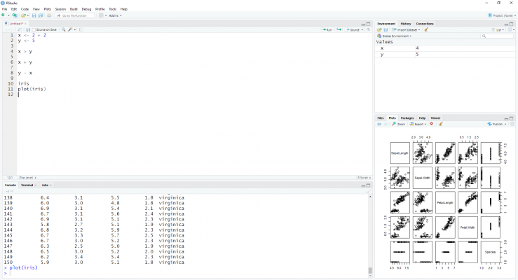
The most popular IDE for R is by some distance RStudio. By default, RStudio is made up of four panes: a source pane where you write the code; a console pane where the code is evaluated; an environment pane where you see your created objects; and a final pane where you can either see the files in your working directory, the plots that are outputted, the packages on your system, or a help screen for documentation.

RStudio offers numerous advantages, which helps make writing R code much easier. For example, you can see the documentation for a package or function by using ? prefix before the name of the package or function. You can use ctrl + R (Cmd+Shift+R on the Mac) shortcut to insert code sections that can be hidden and shown, making the navigation of long scripts effortless. Alternatively, you can chunk up your code by adding four dashes to commented lines of code. You can also automatically format your code by using the ctrl + shift + A shortcut on Windows (Cmd + I on Mac), and much more.

Although base R is substantial, R can be improved by taking advantage of packages. A package is a collection of functions, data, and documentation created by the community which extends the capabilities of base R. Packages are installed for free from the comprehensive R archive network (CRAN) using the install.packages() function, and are loaded using the library() function.

Data Manipulation with dplyr

The dplyr package is an effective library for data transformation and manipulation. It is part of what is known as the Tidyverse – a collection of packages developed by Hadley Wickham that aim to work seamlessly together. Wickham is extremely influential in the R community and has contributed significantly to the development of R.

A debate exists in the R community over whether to use base R or the Tidyverse. It is said that the Tidyverse offers greater readability of code, however, base R is more reliable. Generally, it comes down to personal preference. My advice to beginners would be to learn base R first before looking into Tidyverse packages.

As we know, approximately 80% of data scientists’ time is spent tidying data. Wickham defines data as being tidy when it is in a consistent structure, where each column is a variable, and each row is an observation, allowing you to focus on asking questions with data instead of fighting to get it into the right form for different functions.

Most data manipulation tasks fall within 5 ‘verbs’ that dplyr is built around:

• select() – for choosing certain columns
• filter() – for subsetting rows based on values
• arrange() – for ordering data
• mutate() – for creating new columns
• summarise() – for aggregation

With these verbs, along with functions such as distinct(), count(), group_by(), left_join(), inner_join(), etc. it is easy to see the influence that structured query language (SQL) has had on dplyr. You can even automatically translate your dplyr code into a SQL query, by using the show_query() function. Take this code, for example, the structure is somewhat similar to an SQL query:

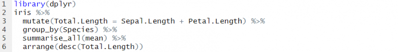
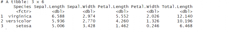
Here, we are querying the iris dataset, we are creating a new column named Total.Length by using the mutate function, we are grouping by species then taking the mean of all columns for each species. Finally, we are ordering the result by our new Total.Length column.

Compare the dplyr code above to the same result using base R code:

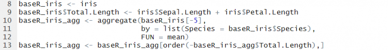
The code that uses dplyr is more understandable, right? This is partly because of the use of %>%, known as pipes. This operator provides a mechanism for chaining commands to help with the readability of code, emphasising the sequence of actions. It can be read as saying “then”.

The output looks like this:

Other commonly used packages for data manipulation include:

• lubridate – for dealing with dates and times
• tidyr/reshape2 – for pivoting and unpivotting data
• stringr – for dealing with character strings
• zoo – for time series data
• scales – for formatting data

With that, I bring this post to a close. In part 2 we look at one of the most recognised capabilities of R, using graphics to communicate data.

References

The R Project for Statistical Computing: https://www.r-project.org/about.html

R for Data Science – Garrett Grolemund and Hadley Wickham

Advanced R – Hadley Wickham: http://adv-r.had.co.nz/

The Tidyverse Style Guide – https://style.tidyverse.org/

Wikipedia: R (programming language) – https://en.wikipedia.org/wiki/R_(programming_language)

A Crash Course in R Part 1 and Part 2– Tristan Robinson (Adatis)