Spark Streaming
Structured Streaming
• Strong guarantees about consistency with batch jobs – the engine uploads the data as a sequential stream.
• Transactional integration with storage systems – transactional updates are part of the core API now, once data is processed it is only being updated, this provides a consistent snapshot of the data.
• Tight integration with the rest of Spark – Structured Streaming supports serving interactive queries on streaming state with Spark SQL and JDBC, and integrates with MLlib.
• Late data support – explicit support of “event time” to aggregate out of order data (late data) and bigger support for windowing and sessions, this avoids the problems Spark Streaming has with Processing Order.
Source Data
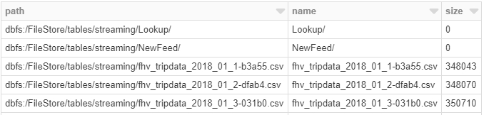
%fs ls "/FileStore/tables/streaming/"
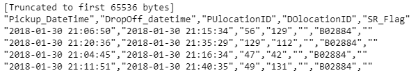
%fs head "/FileStore/tables/streaming/fhv_tripdata_2018_01_1-b3a55.csv"
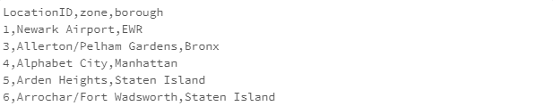
%fs head "/FileStore/tables/streaming/Lookup/NYC_Taxi_zones.csv"
Data Loading
from pyspark.sql.functions import *
from pyspark.sql.types import *
inputPath = "/FileStore/tables/streaming/"
staticDataFrame = spark.read.format("csv")\
.option("header", "true")\
.option("inferSchema","true") \
.load(inputPath) \
.select("Pickup_DateTime", "DropOff_datetime", "PUlocationID", "DOlocationID")
OrderSchema = staticDataFrame.schema
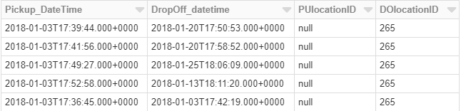
display(staticDataFrame)
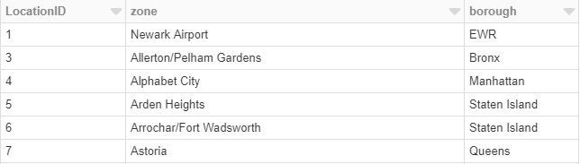
Now let’s load the mapping table for NYC zone and borough names:
LocationPath = "/FileStore/tables/streaming/Lookup/NYC_Taxi_zones.csv"
df_Location = spark.read.option("header", "true").csv(LocationPath)

display(df_Location)
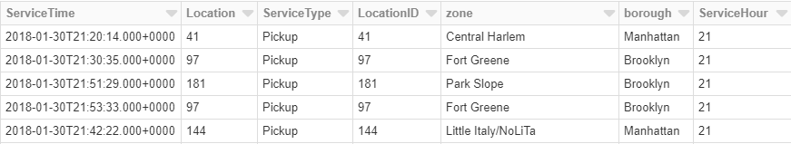
Let’s add some business logic for the purposes of the analysis, we need to combine Pickup_datetime and Dropoff_Datetime in one column – called ServiceTime and adding a new hardcoded column for Service Type. We also need to join our static data frame with the location mapping table to retrieve the borough and zone names.
df_Pickup = staticDataFrame.select(col("Pickup_Datetime").alias("ServiceTime"), col("PUlocationID").alias("Location")).withColumn("ServiceType",lit("Pickup"))
df_Dropoff = staticDataFrame.select(col("Dropoff_Datetime").alias("ServiceTime"), col("DOlocationID").alias("Location")).withColumn("ServiceType",lit("DropOff"))

df_final = df_Pickup.union(df_Dropoff)
df_final = df_final.join(df_Location,df_final.Location == df_Location.LocationID, 'left' ).withColumn("ServiceHour", hour("ServiceTime"))

df_final.createOrReplaceTempView("taxi_data")
staticSchema= df_final.schema

display(df_final)
Now we can compute the number of “Pickup” and “Dropoff” orders per borough, Service hour, Service day with one-hour windows. To do this, we will group by the ServiceType, ServiceHour, ServiceDay and borough columns and 1-hour windows over the Servicetime column.
from pyspark.sql.functions import *      # for window() function
staticCountsDF = (
    df_final\
      .selectExpr( "Borough",
                   "ServiceType",
                   "ServiceHour",
                   "ServiceTime").withColumn("Service_Day",  date_format(col("ServiceTime"),'EEEE'))
        .groupBy(
                     col("Service_Day"),
                     col("ServiceType"),
                     col("ServiceHour"),
                     col("Borough"),
                     window("ServiceTime", "1 hour"))
                .count()
            )

staticCountsDF.cache()
# Register the DataFrame as view 'static_counts'
staticCountsDF.createOrReplaceTempView("static_counts")
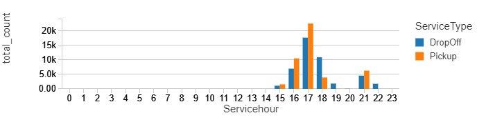
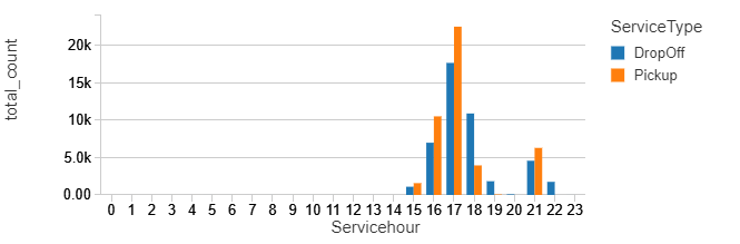
Now we can directly use SQL to query the view. For example, here are we show a timeline of windowed counts separated by Service type and Service hour.
%sql
select ServiceType,Servicehour, sum(count) as total_count from static_counts group by ServiceType,Servicehour order by Servicehour, ServiceType
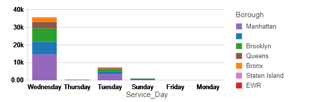
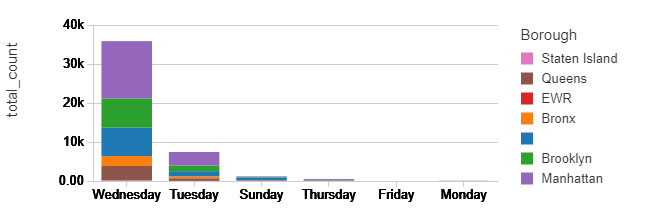
%sql
select Borough,Service_Day, sum(count) as total_count from static_counts where Servicetype = 'Pickup' group by Borough, Service_Day order by Service_Day
from pyspark.sql.types import *
from pyspark.sql.functions import *
spark.conf.set("spark.sql.shuffle.partitions", "2")
streamingDataframe = (
  spark
    .readStream
    .schema(OrderSchema)
    .option("maxFilesPerTrigger", 1) \
    .format("csv")\
    .option("header", "true")\
    .load(inputPath)
)
Let’s add the same logic as before. The result of the last command OrderByBoroughPerDayAndServiceType.isStreaming is true, meaning our streaming is active.
# Let's add some business logic
df_StreamingPickup = streamingDataframe.select(col("Pickup_Datetime").alias("ServiceTime"), col("PUlocationID").alias("Location")).withColumn("ServiceType",lit("Pickup"))
df_StreamingDropoff = streamingDataframe.select(col("Dropoff_Datetime").alias("ServiceTime"), col("DOlocationID").alias("Location")).withColumn("ServiceType",lit("DropOff"))
df_Streamingfinal = df_StreamingPickup.union(df_StreamingDropoff)
# Join Streaming data with location mapping table to retrieve the relevant NYC zone names
df_Streamingfinal = df_Streamingfinal.join(df_Location,df_Streamingfinal.Location == df_Location.LocationID, 'left' ).withColumn("ServiceHour", hour("ServiceTime"))
# Same query as staticInputDF
OrderByBoroughPerDayAndServiceType = (
  df_Streamingfinal
   .groupBy(
     date_format(col("ServiceTime"),'EEEE').alias("Service_Day"),
       df_Streamingfinal.ServiceType,
       df_Streamingfinal.ServiceHour,
       df_Streamingfinal.borough,
       window(df_Streamingfinal.ServiceTime, "1 hour")
          )
    .count()
)
OrderByBoroughPerDayAndServiceType.isStreaming
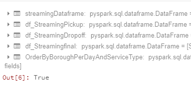
Now we have a streaming dataframe, but it is not writing anywhere. We need to stream to a certain destination using writestream() on our dataframe with concrete options:
spark.conf.set("spark.sql.shuffle.partitions", "2")
query = (
  OrderByBoroughPerDayAndServiceType
    .writeStream
    .format("memory")        # memory = store in-memory table (for testing only in Spark 2.0)
    .queryName("counts")     # counts = name of the in-memory table
    .outputMode("complete")  # complete = all the counts should be in the table
    .start()
)
We can now watch the data streaming live while in our notebook.
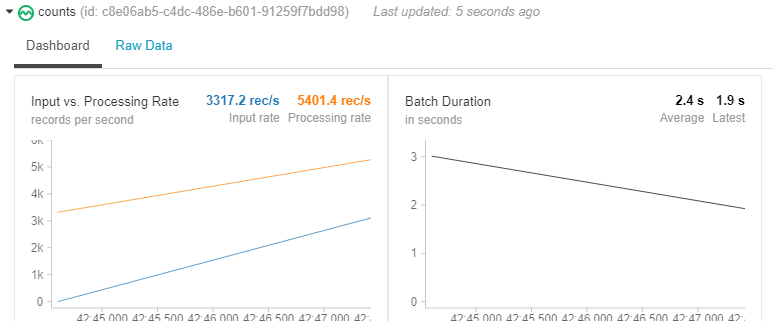
Let’s wait 5 seconds for some data to be processed:
from time import sleep
sleep(5)
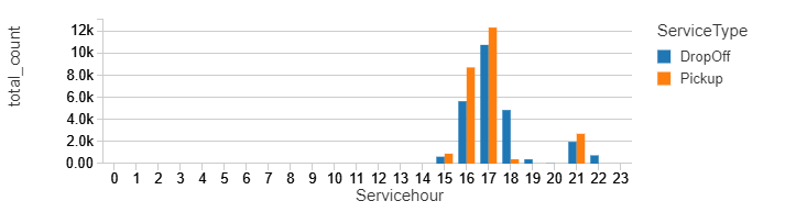
Let display the same charts as we did for our static data:
%sql
select ServiceType,Servicehour, sum(count) as total_count from counts group by ServiceType,Servicehour order by Servicehour, ServiceType
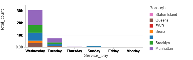
%sql select Service_Day, borough, sum(count) as total_count from counts group by Service_Day, borough
sleep(5)
%sql select ServiceType,Servicehour, sum(count) as total_count from counts group by ServiceType,Servicehour order by Servicehour, ServiceType
%sql select Service_Day, borough, sum(count) as total_count from counts group by Service_Day, borough
Introduction to Data Wrangler in Microsoft Fabric
What is Data Wrangler? A key selling point of Microsoft Fabric is the Data Science
Jul
Autogen Power BI Model in Tabular Editor
In the realm of business intelligence, Power BI has emerged as a powerful tool for
Jul
Microsoft Healthcare Accelerator for Fabric
Microsoft released the Healthcare Data Solutions in Microsoft Fabric in Q1 2024. It was introduced
Jul
Unlock the Power of Colour: Make Your Power BI Reports Pop
Colour is a powerful visual tool that can enhance the appeal and readability of your
Jul
Python vs. PySpark: Navigating Data Analytics in Databricks – Part 2
Part 2: Exploring Advanced Functionalities in Databricks Welcome back to our Databricks journey! In this
May
GPT-4 with Vision vs Custom Vision in Anomaly Detection
Businesses today are generating data at an unprecedented rate. Automated processing of data is essential
May
Exploring DALL·E Capabilities
What is DALL·E? DALL·E is text-to-image generation system developed by OpenAI using deep learning methodologies.
May
Using Copilot Studio to Develop a HR Policy Bot
The next addition to Microsoft’s generative AI and large language model tools is Microsoft Copilot
Apr