Introduction to Spark-Part 2:Jupyter Notebooks

This is the second post in a series on Introduction To Spark.

What Are They?

Jupyter Notebooks provide an interactive environment for working with data and code. Used by Data Analysts, Data Scientists and the like, they are an extremely popular and productive tool. Jupyter Notebooks were previously known as IPython, or ‘Interactive’ Python, and as such you will still find reference to this name throughout various documents.

The Notebook Environment

The Jupyter notebok environment consists of a browser-based notebook UI and a back-end server, running on port 8888 by default (if this port is taken it will start up on the next available port). This web server-based delivery of Notebooks means that you can browse to a remote server and execute your code there. This is the case, for example, when using a ready-made cluster such as an HDInsight Spark cluster, where all the tooling has been pre-installed for you. You open the notebook in the cluster portal within Azure, and it logs you in to the Jupyter server running on a node within the cluster. Note that if you want to allow multi-user access to your local Jupyter environment, you’ll need to be running a product such as JupyterHub.

Starting the Notebooks Environment

For our local install, we can run our Jupyter Notebooks using a couple of different methods

Anaconda Jupyter Notebook

As mentioned in the previous post, Anaconda comes with Jupyter pre-installed. For each Python Environment that you have the Jupyter Notebook package installed to, you will see a Jupyter Notebook() entry under the Anaconda Start menu items. You can also access this from the Anaconda Navigator Home tab, together with a bunch of other Data Analytics-related applications such as rstudio and spyder.

Conda Prompt

Open an Anaconda Prompt, change to the required environment and execute the application:

Activate 
Jupyter Notebook

This will execute the jupyter-notebook.exe file (via the Jupyter.exe file) installed within the selected environment, being the entry point for the Jupyter Notebook application.

It is important to load the installation of Jupyter Notebook in the desired Python environment in order to have access to kernels that have been installed there.

Shutting Down the Jupyter Server

You can close your Jupyter Notebook at any time, but you will need to make sure that the server process has also stopped. Back in your command window, press Ctrl+C twice, and it will shutdown. This will return you to the command prompt.

Kernels

The code you enter in your notebook is executed using a specified kernel. There are a whole bunch of kernels supported, as detailed here, which can be easily installed into the environment and configured as required. The most popular kernels for working with Spark are PySpark and Scala. I’ll take you through installing some of these kernels in the next post in the series.

Cells

Jupyter notebooks consist of cells, in which you enter code for your data analytics needs for number crunching and rendering visuals, write markdown text (for documentation) and even add basic UI controls such as sliders, dropdowns and buttons. Your code will use the chosen kernel and as such must comply with the respective execution language. This offers a very productive collaboration environment in which to work, with the notebooks containing the instructions to calculate and visualise the data of interest being easily shared amongst co-workers. They may appear at first to be a bit basic, but in reality they offer pretty much everything you need to get to grips with analysing and displaying your data, leveraging all manner of libraries within your chosen language.

Cell output can be in ASCII-text rendered tables, formatted text, or various visualisations such as formatted tables, histograms, scatter charts or, if you tap into the more advanced widgets/tools, animated 3D graphs and more.

Edit Mode vs Command Mode

These two modes offer different behaviour within the notebook. ‘Edit mode’ is for editing within your cells, ‘command mode’ for issuing commands that are not related to cell editing but more to the notebook itself. To enter ‘edit mode’, simply press Enter on a cell, or click within the cell. To leave ‘edit mode’ and enter ‘command mode’ press Esc. On executing a cell, you will automatically enter ‘command mode’.

Keyboard Shortcuts

There are a considerable number of keyboard shortcuts within the notebook environment, the list of which can be seen by clicking on the ‘command palette’ button. Some commonly used shortcuts of note are:

Function Shortcut Description Run Cell and Select Next Shift + Enter (Edit Mode) This executes the current cell and moves to the next one. Run Cell and Insert Next Alt + Enter (Edit Mode) This executes the current cell and inserts a new cell below the current one. Run Selected Cells Ctrl + Enter (Edit Mode) This executes all currently selected cells. Delete Cells d d This deletes the currently selected cell. Cut Selected Cells x (Command Mode) Cuts the selected cells to the clipboard. Copy Selected Cells c (Command Mode) Copies the cells to the clipboard. Paste Selected Cells below v (Command Mode) Pastes the cells from the clipboard to the notebook below the current cell. Paste Selected Cells above Shift + v (Command Mode) Pastes the cells from the clipboard to the notebook above the current cell. Select Next, Previous Cell Up, Down (Command Mode) Moves to the cell above or below the current cell.

It’s worth familiarising yourself with the various shortcuts of course as an aid to productivity.

Magics

Magics are essentially shortcut commands for various actions within the Jupyter Notebook environment. The magics auto-loaded will depend on the kernel chosen. Magics come in two flavours, cells magics and line magics.

Cells Magics

These are prefixed %% and act on the contents of the cell

Line Magics

These are prefixed % and act on the contents of the line that the magic is on. If the ‘Automagic’ functionality is turned on, the % is not required.

Many magics have both cell and line versions.

Viewing Magics Available in the Kernel

You can list the magics available using, yep, you guessed it, a magic. %lsmagic will show all cell and line magics currently loaded. If you require loading another magic, use the %load_ext . You should consult the specific magic documentation in order to get the correct reference to use for loading with %load_ext. You can get help on a specific magic by typing %?

Common Magics

%load_ext

As mentioned, this will load a magic up from a library, providing it has been installed in the respective kernel environment.

%config

This allows configuration of classes made available to the IPython environment. You can see which classes can be configured by executing %config with no parameters. We’ll make use of this for the %%read_sql magic below.

%%SQL

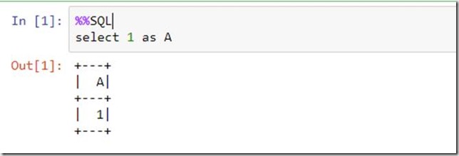
Probably the most commonly used within Spark is the SQL Magic, %%SQL. This allows using SparkSQL with a SQL syntax from within the notebook, reducing the code written considerably. It is available within the Spark Kernel installed within Apache Toree, so you will need to start the ‘Apache Toree – Scala’ kernel to use this magic.

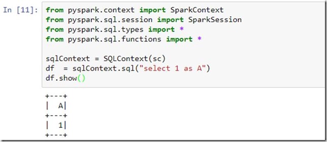
With SparkSQL you would ordinarily write something along the lines of

but with the %%SQL magic, this simply becomes

It basically returns a Spark DataFrame from the SQL expression used, and renders it to the results area under the cell. Given the power that SparkSQL has (as we’ll see in a later post) this simplifies use of that most popular of data querying languages, namely our good old friend SQL.

%read_sql, %%read_sql

If you are using a different kernel, you will need to use an alternative, such as %read_sql from the sql_magic package supplied by Pivotal, which requires a little more code. You can read about installing and using that here.

To use this with Spark, you will need to connect to the Spark Context. This is done by changing a configuration property for the conn_name property of the sql config class to ‘spark’. After installation, you’ll need to use the following boilerplate code:

You can then use the magic as below:

Slightly different output style, but essentially the same as %%SQL.

%%HTML

Pretty obvious this one. Will output your HTML to the results area under the cell, allowing display of webpage content within the notebook

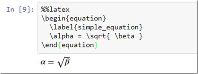
%%Latex

For those writing equations or requiring the formatting commonly found in scientific papers, this offers a subset of LaTex functionality as provided by MathJax.

Rather spiffing considering all the maths generally kicking around on your average Data Science project.

Notable Packages for Installation

Below are a few packages of note. You can install these into your python environment using pip install or the Anaconda Navigator environment package manager (please see previous post for information on this) or conda prompt. When using pip you will need to enable the extension as well. The extension does not necessarily share the same name as the package installed, so check the respective documentation for installation specifics. For example, installing IPyWidgets requires running the following:

pip install ipywidgets
jupyter nbextension enable --py widgetsnbextension

IPyWidgets

A set of core Ipython/Jupyter widgets that include a bunch of controls, such as the Slider for selecting numeric values, Dropdown, Command Button etc. You can build a rudimentary UI in your notebook with these, at least for your data filtering/selection purposes. See here for some examples.

This package is a dependency for various other packages, such as AutoVizWidget.

AutoVizWidget

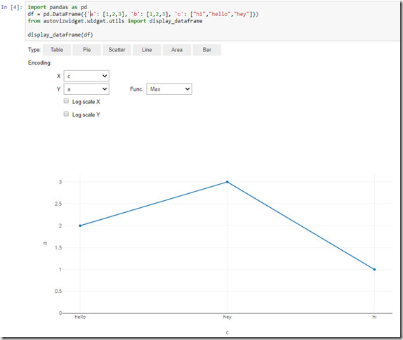
This provides simple visualisation of pandas data frames, with controls to change the visualisation type. You’ll see these controls pre-installed in the HDInsight installation of Jupyter Notebooks.

You can see examples of usage here. This uses the Plot.ly library. As you can see this allows very quick visualisations with some easy options for changing displays.

Plot.ly

An advanced data visualisation library, with some pretty impressive display options and requiring a relatively small amount of code input. You can find an introduction here.

See the Visualisations section below for an example usage, and note that you don’t have to create an account to use this, just use the plotly.offline objects.

Dash

Also from Plot.ly, this has some serious visual capabilities. It is a commercial venture from Plot.ly but is available for free if you don’t need the distribution platform for Enterprise use. To use within Jupyter however you will need to use an HTML element to embed it in an iframe. I haven’t played with this one yet, but you can find out how this is apparently done here.

Visualisations

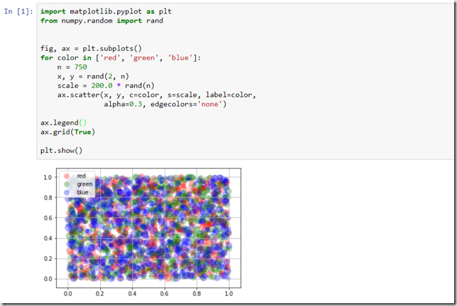
It is easy to quickly output visuals when working with pyspark, using libraries such as matplotlib, plotly(based on matplotlib) and others. Simply import the required packages, prepare a dataset for rendering and with a few simple lines of code you have your data displayed.

Matplotlib

The foundation for pretty much everything else for numerical visualisation, this allows Pandas data frames to be rendered in a very succinct fashion. Installation instructions are here, with a dizzying number of examples here.

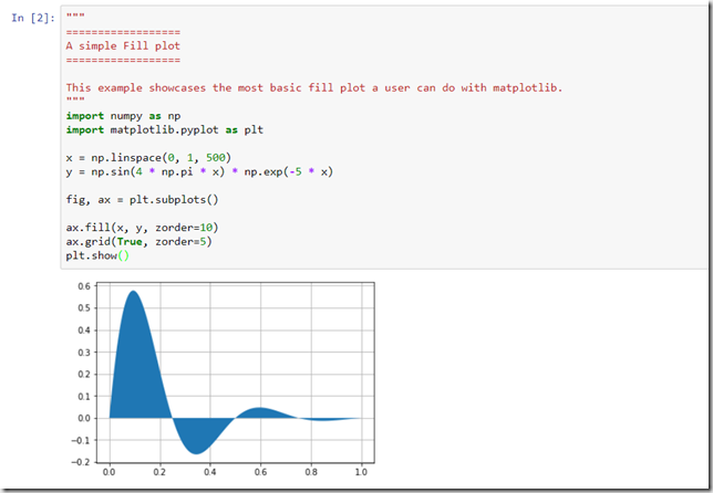
Here’s another example, not so much of an impressionist style…Sinusoidal with exponential decay (dampened Sinusoid).

Plot.ly

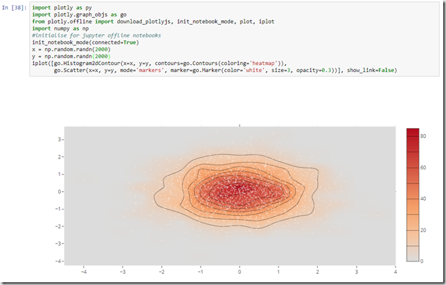
Here’s a quick example of a Histogram 2D Contour with heatmap colouring. Not bad for less than 10 lines of code (although it does look like it might double as a secret base for a Bond villain).

 

Troubleshooting

Below are a couple of common issues you may encounter when running Spark locally with Jupyter Notebooks.

Apache Derby lockouts

The default hive metastore used under the covers by Spark will run on Apache Derby, which is a single user connection database. So if you try and fire up another process that wants to access this, you will receive an error similar to that below:

Caused by: ERROR XJ040: Failed to start database ‘metastore_db’ with class loader org.apache.spark.sql.hive.client.IsolatedClientLoader$$anon$1@1dc0ba9e, see the next exception for details.

at org.apache.derby.iapi.error.StandardException.newException(Unknown Source)

at org.apache.derby.impl.jdbc.SQLExceptionFactory.wrapArgsForTransportAcrossDRDA(Unknown Source)

… 107 more

Caused by: ERROR XSDB6: Another instance of Derby may have already booted the database C:WindowsSystem32metastore_db. at org.apache.derby.iapi.error.StandardException.newException(Unknown Source)

…

The path above to the metastore will depend on where your current working directory is, so may well be different. The lock file db.lck should clear when shutting down the other notebook instance, but if it doesn’t you are okay to delete it as it will be created on each connection. For ‘real’ installations you should be using a different database for the metastore, such as MySQL, but for personal experimentation locally this is not really necessary.

Hive Session Creation Failed

As per the previous post you may encounter this due to permissions on the tmphive directory. Please see the previous post for a solution to this issue.

Next up…

In the next post in the series we’ll look to extending Jupyter Notebooks by Installing Jupyter Kernels.