Improving Machine Learning Models

As part of my MS Data Science Professional Program, a number of the topics recently have been based around getting the most out of an Azure ML model. As part of this blog, I will be looking at the techniques and ways in which you can model and improve a solution. While I was tackling this problem with Azure ML, these techniques apply to building better models through other languages/platforms such as Python or Scala.

Data Munging

A process that undoubtedly every data scientist goes through with every DS problem they face, is that of data munging. This is a term that is being used more frequently to describe the process of transforming data from its raw state into another format, something more valuable for downstream analytics. Models running on data that is poor in quality, missing or duplicated will produce poor predictions. Therefore a very simple pre cursor to any problem is to explore the data and understand what is required to turn the data set into a form which is better for the latter stages of the model design. The following techniques are used as part of this stage:

• Removing Duplicate Rows
• Cleaning Missing Data (custom substitution of numerics, usually 1 or 0 or replacing with the mean, medium, mode across the dataset)
• Cleaning Missing Data (removing bad quality rows entirely or removing bad quality columns entirely – more extreme)
• Creating Categorical Features from String Features
• Normalising Numeric Features (ZScore or Min/Max) to bring everything on to the same scale.

These steps are quite basic so I won’t go into detail here, but none the less, they should be considered at the start of a modelling a better solution to a problem.

Feature Selection

One of the reoccurring principles that appears with machine learning is that of Ockham’s razor, which states that the best models are simple models that fit the data well; this is not an irrefutable principle of logic, but a preference for simplicity. Therefore there is a need of balance between accuracy and simplicity to limit the feature set which tends to lead to better predictions. Simpler models are also more interpretable to humans which also helps. While the data I was working with was limited to around 35 features, there are many data science problems which have thousands of features and so this technique is even more crucial.

There are multiple methods to perform feature selection, of which a few will be covered here. The first method is greedy backward selection which starts with all the features and then finds the feature that hurts predictive power the least when removed, and you remove it. This is done iteratively until a point is met (which will be discussed later). Its known as greedy since it never looks back after removing the feature each time.

An alternative method is greedy forward selection which is basically the inverse, starts with no features, and looks for the feature that by itself is the best model. This then carries on in a similar vein to the backward selection but adding features. The point at which you stop with forward selection is that of diminishing returns for your accuracy.

Defining accuracy is important here, and this is where a formula called Adjusted R? comes in. R? is a measure of how well the model fits the data, with being closer to 1 than 0 being a better fit. The adjusted part adds a penalty for every term in the model, thus it measures on a scale the size and accuracy of a model. Therefore you need enough features for your R? to be large but not too many that it brings the Adjusted R? down.

.

Permutation Feature Importance

Using the feature selection theory, and to prune the feature set down to those that are meaningful for prediction, you can use a module in Azure ML called Permutation Feature Importance. This essentially re-computes the model a number of times, leaving out each feature and looks at how much your metric changes because the feature was left out, and then ranks them in order of importance. Depending on what you are trying to model, i.e. a classification or regression problem – there are a number of options for the metrics to measure performance. In my instance, I was interested in the RMSE (Root Mean Squared Error) which in simple terms represents the sample standard deviation of the difference between prediction and observed values. It aggregates the magnitudes of error in prediction into a single measure of predictive power. The closer to 0, the better the predictive power – but it’s also good to note this is relative to what you are trying to measure.

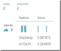
Once the model has been run through, you can visualise the list of features and their contribution to the RMSE. At this point, it does not necessarily matter whether the feature contributes a positive or negative value to the RMSE, as long as the value is not 0. Any values of 0 indicate that they have zero contribution to feature importance, essentially whether they are part of the model or not, add nothing to it. You can then follow backward pruning techniques to remove these columns from the feature set. It is then worth running the model again, to check the feature importance as the removal of those features may impact other features. If more features then have a value of 0, you should remove those too, and repeat. You can then measure the impact of the changes using separate pipelines, and passing the output into the same evaluation model, and checking the ROC curve (described below). Even with the RMSE staying the same between the 2 pipelines, by removing features, you are able to build a model which is more likely to generalize – be more effective in the real world when values change.

Picking the Best Model Type

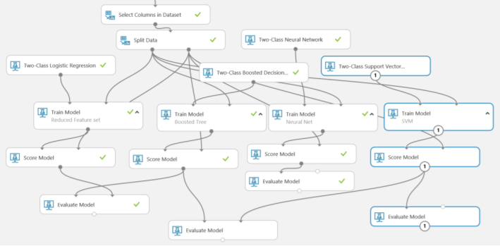
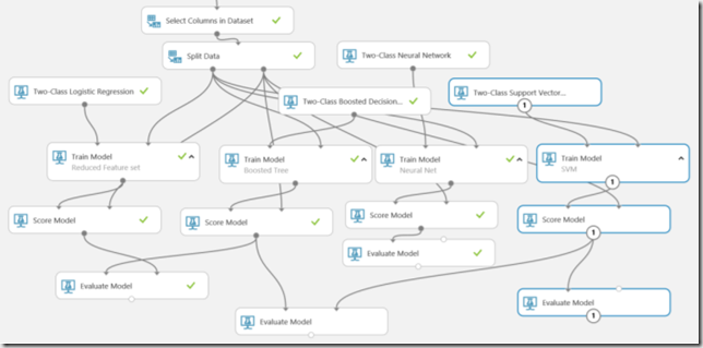
There is no reason to believe that any particular machine learning model will have the best performance (although we always have favourites); a classification model type that works best for one set of features and labels in a dataset does not always work best for another. As part of modelling any dataset, testing and comparing multiple machine learning models is usually a good approach. Its also important to note that the performance achieved with any particular machine learning model can change after performing feature engineering, therefore it is best to run the selection after this stage. The following model evaluates logistic regression, boosted decision trees, neural networks and support vectors with the same dataset to find out which is best.

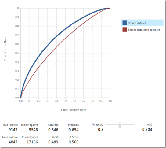
To understand the performance of a machine learning model, there are a number of techniques to use. The easiest way is to pass the output of each model into an Evaluate Model module, which accepts up to 2 datasets at a time (left and right inputs). After the experiment is run, you can visualise the output of the models using this module, and examine the ROC curve. The first scored dataset (blue) represents the original model (in this case a neural network), and the scored dataset to compare against (red) represents the second dataset (in this case a support vector machine). The higher and further to the left the curve, the better the performance of the model (in this case, the neutral network).

Scrolling down further, you can also use the Accuracy, Recall, and AUC performance metrics, which indicate the accuracy and area under the curve. The model with the higher metrics is performing better. In particular, the lower the recall metric, the higher the number of false negatives.

Parameter Sweeping

Once you’ve picked the ML model contributing to making your predictive power better, it will require a set of parameters. For instance, with decision trees, this is in the form of a leaf count to determine depth, or no. of trees to determine width, along with their samples per leaf, and the learning rate. By default there is always a set available, but these will always need tweaking to improve things further and generate a better RMSE.

This can be done by either sweeping a giant grid of parameters, or by a random sweep. The latter being a lot quicker to process at run time for obvious reasons Fortunately, the performance is not normally sensitive to a change in these values if you have done much of the previous analysis first. Parameter sweeping really starts to squeeze the best out of the model.

In Azure ML, this can be done via a tune model hyper parameter module. The same options are available to measure metrics as the feature selection module, so I was interested in the RMSE again. As part of tuning the parameters through this module, we will need to split the training data beforehand, this can be done 50:50. This is so that the parameters have a set of data to validate against. This is then kept separate to the scoring data set as usual which is another completely separate set of data. Once the model has run, we can again evaluate the best parameters, against the original model and evaluate the RMSE, as well as the Accuracy, Recall and AUC. This is very similar to the previous techniques of evaluation. Visualising the sweep results, will display the parameters used, and then these can be programmed back into the original ML model, while removing the tune hyper parameter module, to speed things up on future runs.

A process of nested cross validation can be used on top of this to build confidence that the correct parameters have been used and it wasn’t just luck that they ended up being better than another set.

Conclusion

Once you have been through this process, you will then want to run a process of cross-validation, which runs the data through multiple times (folds) where each time, different data is used for training, and scoring. You can then generate a mean and standard deviation for each fold and prove the model is consistent across the data set, and that it will not be skewed by any new data for future predictions. This will give you a good idea of whether the model will generalise well and be robust enough to move to production.

Of course, there are many more techniques to the ones listed here, but this should give you a good introduction to the ones to look for to deliver predictive power from your model.