Programming languages such as Python and MATLAB can be used to build many different kinds of models. However, these languages can be difficult for some to grasp as they require a solid understanding of programming concepts and syntax – which may be challenging for beginners or those with limited programming experience. Hence, it may sometimes be more practical to build these models using applications which have a lower barrier to entry. This not only better facilitates model development in these circumstances, but also consumption/comprehension by senior stakeholders.

This blog will focus on Microsoft Power Query as a means of building models. Power Query is a data transformation and preparation tool that enables users to easily manipulate data using a graphical user interface, GUI (or programmatically, using a language called M, if required). Normally, users use a variety of transformation processes to clean data in Power Query. However, these same transformation processes can also be used to build models in some cases! In these cases, the implementation in Power Query is often much simpler than the would-be implementation in languages such as Python or MATLAB. Let’s explore an example.

Example and Problem Statement

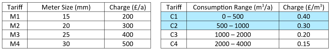
Wotter Inc. provides water to households and organisations, which are charged based on how much water they consume, or, if this quantity is unknown, their meter size.  The tables below show the meter and consumption-based tariffs:

Also, the Customer Information table is required and is shown below:

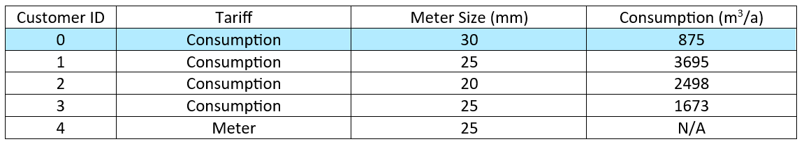
Your manager has tasked you with calculating the bill for each customer. For customers charged based on consumption, you are to compare two options (as illustrated below using Customer 0 – please refer to the highlighted rows in the tables).

Option 1: Consumption charge is solely based on which ever band customer falls in.

875 x 0.30 = £262.50

Option 2: Consumption charge is based on the summation of volume increments which fall within different bands – this is the same tariff structure that is applied to income tax within the UK.

(500 x 0.40) + ([875 – 500] x 0.30) = £312.50

Example Solution

Meter Size

Calculating the charge for each customer based on meter size can be very simply achieved in Power Query using the following process:

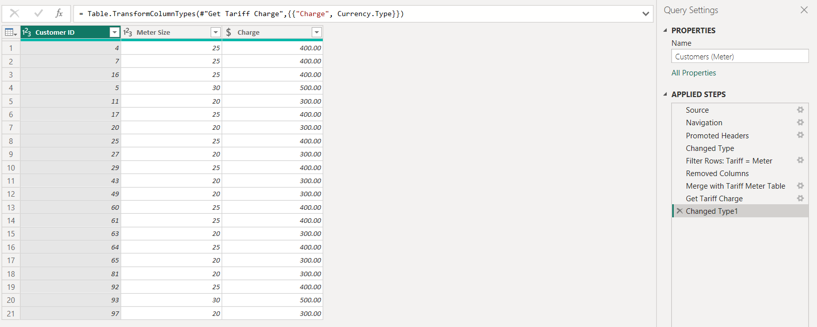
1. Filter the Customers Table to only show rows where Tariff = “Meter”.
2. Use a LEFT OUTER JOIN to join the Customers and Tariff Meters table on Meter Size to return the associated charge for each customer.

Both of these steps can be easily configured using the GUI provided by Power Query. Also, Power Query automatically breaks down the individual steps in the APPLIED STEPS section, providing transparency, reproducibility, and easy modification of data transformations, facilitating model development.

Consumption – Option 1

Calculating the charge for each customer based on consumption using Option 1 can be achieved in Power Query using the following process:

1. Filter the Customers Table to only show rows where Tariff = “Consumption”.
2. Perform a CROSS JOIN to join the Customers and Tariff Consumption tables.

Step 2 results in the following table for Customer 0:

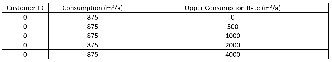
This data structure allows us to identify which consumption band Customer 0 is in. As shown previously, this should be where Upper Consumption Rate is 1000 m³/a.

3. Add a conditional column to check if Consumption < Upper Consumption Rate.
4. Filter the Customers Table to only keep rows where the above returns TRUE.

Steps 3 and 4 result in the following table for Customer 0:

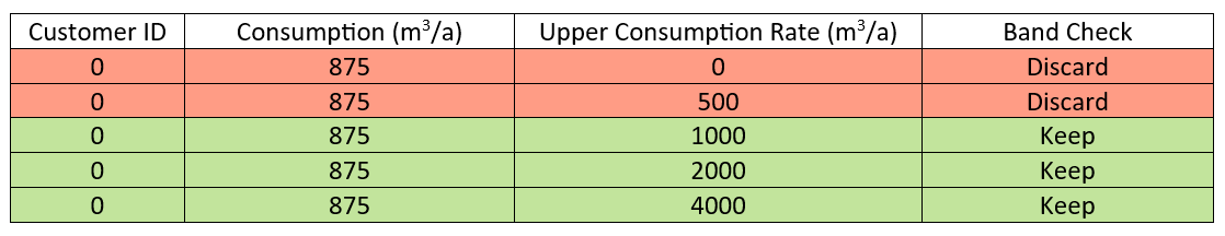
However, as stated previously, we only want to keep the row where Upper Consumption Rate is 1000 m³/a for Customer 0. It is important to note two things:

• This will always relate to the first Keep value as this is where the cross-over occurs.
• Power Query runs these calculations for all Customer IDs – only one is shown for brevity.

Therefore, to return the first Keep value for each customer:

5. Group the Customer Table by Customer ID and Consumption.
6. Add an Index to each group (using the M code situated above the table in the following image) and expand the group.

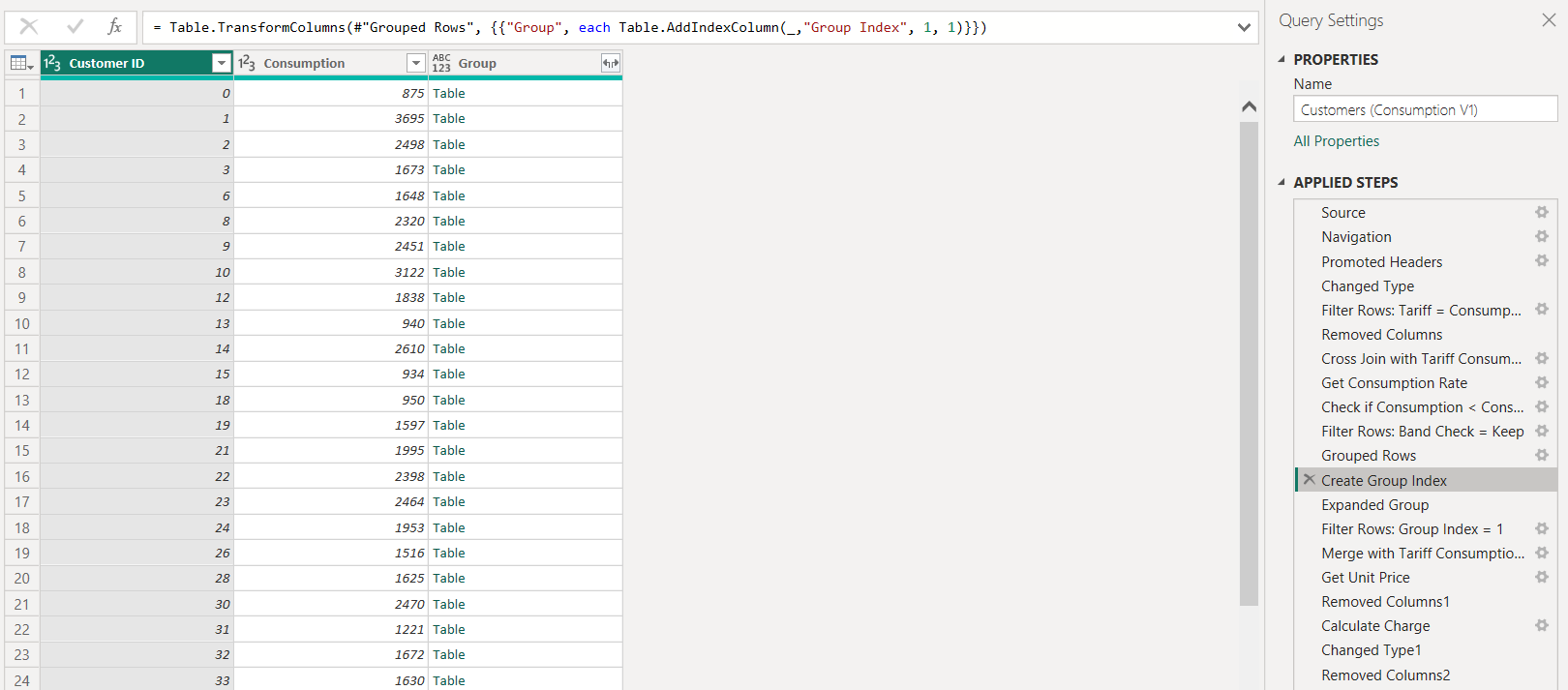
Steps 5 and 6 result in the following table for Customers 0 and 3.

7. Filter the Customers Table to only return rows where Group Index = 1.

Now, you can repeat the same process as applied in the Meter Size section to calculate the charge based on Consumption – Option 1. Specifically:

8. Perform a LEFT OUTER JOIN to join the Customers and Tariff Consumption table on Upper Consumption Rate to return the associated unit price for each customer.
9. Calculate the charge by using the following formula:

Charge = Consumption x Unit Price

Consumption – Option 2

Calculating the charge for each customer based on Consumption using Option 2 is slightly more convoluted than Option 1, however, uses the same methodology. It can be achieved in Power Query using the following process:

1. Repeat Steps 1 to 7 in the Consumption – Option 1 case.

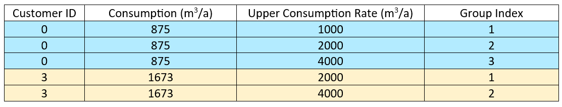
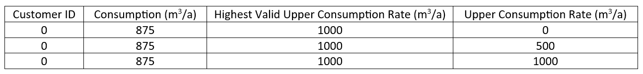
This results in the following table for Customer 0:

Note, the column heading: Highest Valid Upper Consumption Rate. This is because, unlike the Consumption – Option 1 case, the charge is a function of multiple Upper Consumption Rates. For now, we won’t utilise the Highest Valid Upper Consumption Rate column, however it will be utilised later on.

2. Perform a CROSS JOIN to join the Customers and Tariff Consumption tables.

This results in the following table for Customer 0:

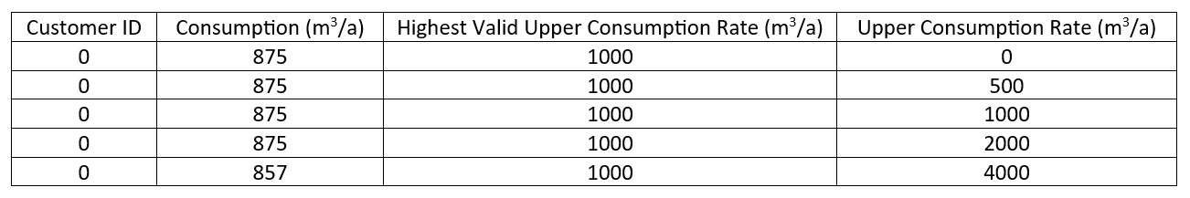
3. Add a conditional column to check if Highest Valid Upper Consumption Rate <= Upper Consumption Rate.
4. Filter the Customers Table to only keep rows where the above returns TRUE.

Steps 3 and 4 result in the following table for Customer 0:

To calculate the charge associated with each band, we need to know the volume consumed within each band. For example, Customer 0 consumes 500 m³/a within Tariff C1 and 375 m³/a within Tariff C2. Therefore, we need to be able to relate rows within the Upper Consumption Rate column to their previous row. This is illustrated below:

Volume Increment Tariff C1 = 500 – 0 = 500 m³/a

This can be done in multiple ways, one of which is the following:

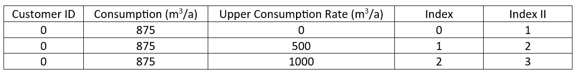
5. Add an index column that starts at 0 with an increment of 1.
6. Add a second index column that starts at 1 with an increment of 1.

This results in the following table for Customer 0:

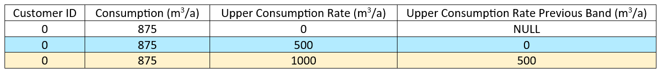
7. Perform a LEFT OUTER JOIN to join the Customers Table to itself.

This results in the following table for Customer 0:

There is now only one more thing to do before we can calculate the volume increments for each band. We need to find a way to represent the following:

⬛︎ Volume Increment Tariff C1 = 500 – 0 = 500 m³/a ✓

⬛︎ Volume Increment Tariff C2 ≠ 1000 – 500 = 500 m³/a ☓

⬛︎ Volume Increment Tariff C2 = 875 – 500 = 375 m³/a ✓

This can be done in the following way:

8. Add a conditional column to check if Highest Valid Upper Consumption Rate = Upper Consumption Rate (for Customer 0, this value is 1000 m³/a).
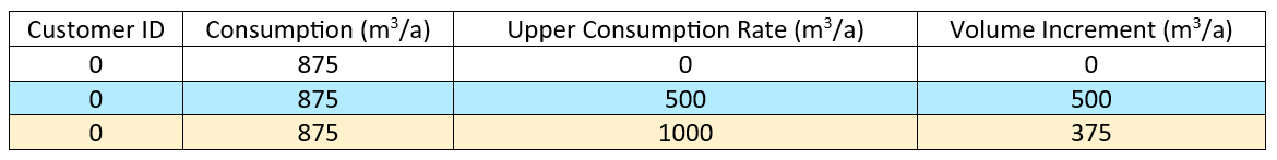
9. Calculate the Volume Increments using the following logic applied to each row:

IF Highest Valid Upper Consumption Rate ≠ Upper Consumption Rate

THEN Upper Consumption Rate – Upper Consumption Rate Previous Band ⬛︎

ELSE Consumption – Upper Consumption Rate Previous Band ⬛︎

10. Due to the chosen method, some rudimentary cleaning steps are required at this stage. In general, these will vary depending on your chosen method of model development.

This results in the following table for Customer 0:

Now, you can repeat the same process as applied in the Consumption – Option 1 section to calculate the charge based on Consumption – Option 2. Specifically:

Volume Increment Charge = Volume Increment x Unit Price

11. Perform a LEFT OUTER JOIN to join the Customers and Tariff Consumption table on Upper Consumption Rate to return the associated unit price for each volume increment.
12. Calculate the charge for each volume increment by using the following formula:
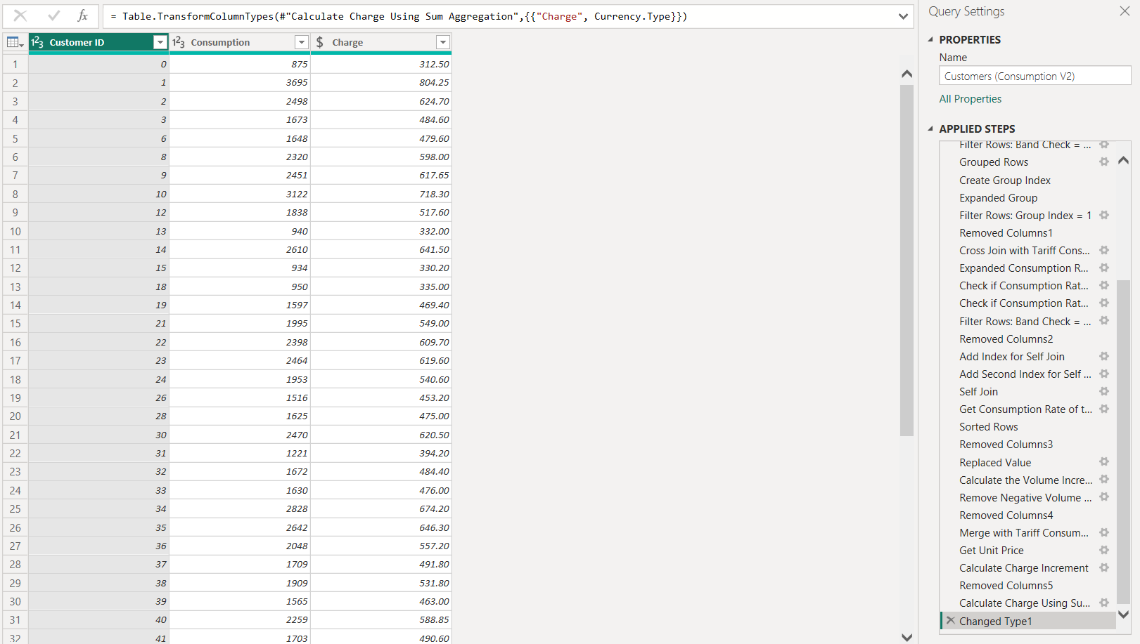
13. Calculate the total charge by aggregating the data. To do this, group by Customer ID and Consumption and create a new column as requested to sum the Volume Increment Charge column.

See the image below to view the final data and applied steps within power query.

Final Thoughts

Power Query is a powerful tool which can be used beyond the conventional data preparation and cleansing use case. As this blog illustrates, we can use Power Query to build complex models, replacing the requirement to use other, more difficult to learn, applications such as Python or MATLAB in some cases. In our example, we used Power Query to build a complex model using a series of relatively basic transformations that included filtering the data, joining tables to each other, creating columns, using IF statements, etc. What makes Power Query so easy to use is that the vast majority of these transformations can be configured using the GUI. It should be highlighted that:

• As with any modelling exercise, there are multiple ways of arriving at the same result, and this blog only illustrates one possible path.
• This blog only illustrates a singular example scenario, the methodologies illustrated in this blog can be applied to a wide range of different scenarios.

In summary, Power Query provides the ability to build complex models whilst being very user-friendly through its GUI, better facilitating the development, consumption and comprehension of models.

Notes

The Power Query model discussed in this blog can be found here.

If you have any questions related to this post please Get in touch and speak to a member of the Adatis team to discuss the topic in greater detail.