Databricks: Cluster Configuration

Databricks, a cloud-based platform for data engineering, offers several tools that can be used to create and configure clusters to achieve the greatest performance for the least amount of cost.

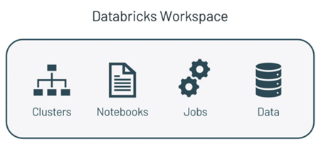
Figure 1 – Databricks tools

In essence, a cluster is a group of virtual machines. A Driver node often coordinates the work done by one or more worker nodes in a cluster. Through the Driver node, clusters enable us to handle this collection of machines as a single computation engine. We may execute a variety of workloads on Databricks Clusters, including ETL for Data Engineering, Data Science, and Machine Learning workloads.

This article will look at the cluster’s high-level configuration and address six topics:

1. Single-node clusters
2. Multi-node cluster
3. Instance pool
4. Cluster optimisation for ADF parallelism
5. Autoscaling clusters
6. Cost management

Types of Databricks Clusters

Azure Databricks offers two primary cluster types: single-node and multi-node clusters, each of which is designed to meet certain workload needs. Single-node clusters provide a low-cost, low-resource computing option for light-duty applications or development work. Multi-node clusters, on the other hand, are perfect for demanding workloads since they distribute tasks across numerous nodes for enhanced performance and capacity, offering scalable computational capability. Azure Databricks gives you the freedom to select the cluster type that best meets your requirements, whether you’re using it for large-scale analytics, algorithm development, or data exploration.

1. Single-node Cluster Configuration

A computational resource made up of only the Apache Spark Driver and no workers is called a single-node cluster. All Spark tasks and data sources are supported. For some lightweight exploratory data analysis tasks and single-node machine learning workloads, single-node computers might be useful.

• Purpose: When processing tiny amounts of data or carrying out non-distributed tasks, single-node clusters are intended for use in particular situations.
• Application cases: For lightweight jobs, a single-node cluster is suitable for activities requiring less data processing or single-node machine learning libraries.

Data exploration and ad-hoc analysis are the perfect uses for these clusters, which are also great for development.

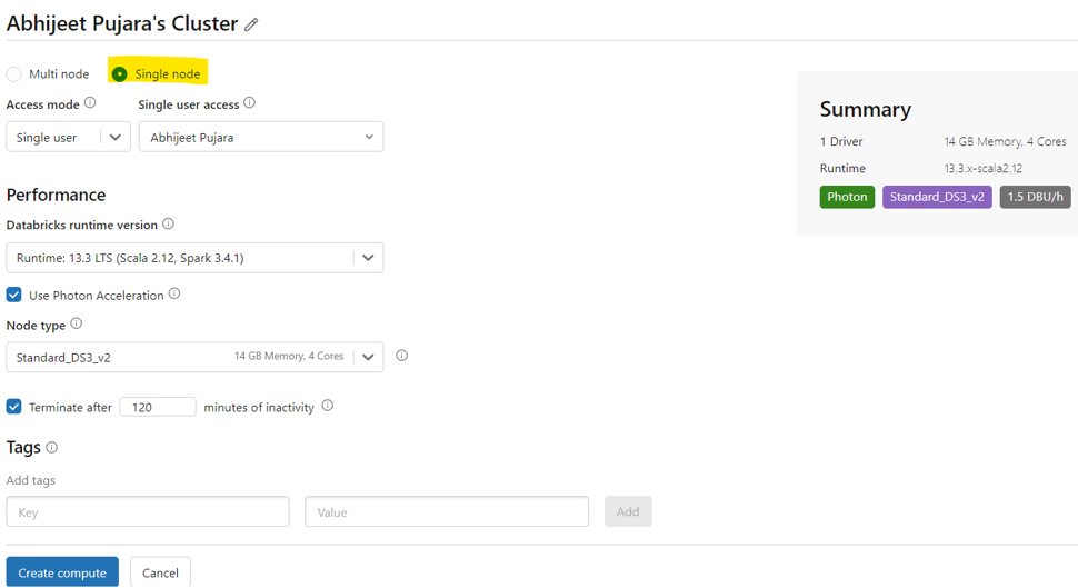
Figure 2 – Single-node cluster configuration

Properties

• Runs Sparks locally
• No worker nodes
• Single-node cannot be converted to multi-node compute.

Limitations

Resource restrictions: Single-node clusters are not designed to be shared. They work well for solitary jobs and offer restricted resources.

Termination: Until they are formally ended, single-node clusters continue. You can also configure them to stop after several idle minutes. In this instance, we set a 120-minute timer.

Process isolation is incompatible with single-node computing. Computers running on a single-node do not support GPU scheduling.

2. Multi-Node Clusters Configuration

One driver node and one or more worker nodes make up a multi-node cluster. The Driver node distributes tasks to the worker nodes to execute in parallel when the Spark job runs against a multi-node cluster. It then provides the results. Depending on the demand, we may scale out the clusters by adding new clusters to the node. These kinds of clusters are appropriate for heavy workloads and are utilised for Spark Jobs.

The goal of multi-node clusters is to handle heavier workloads requiring distributed processing. This provides significant benefits to users:

• Large-Scale data processing: Multi-node clusters are crucial when working with distributed workloads or large amounts of data
• Analytical workloads: Multi-node clusters can handle the processing power required for intricate analytical activities like extract, transform, and load (ETL) operations
• Resource sharing: Multiple users may share access to multi-node clusters
• Termination: Multi-node cluster-based job clusters automatically end a task when it’s finished, saving money and resources
• Cost consideration: Although increased resource consumption influences costs, multi-node clusters provide more power.

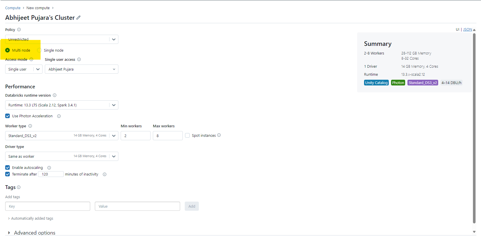
Figure 3 – Multi-node clusters configuration

Access Mode

There are three types of access modes within Databricks clusters:

1. Single User Access Mode: There is only one user who can access the cluster while using the single user access mode. The four languages are supported are Scala, R, SQL, and Python.
2. Shared Access Mode: This allows a cluster to be shared by several users and offers process separation. Every process has its own environment, preventing any one process from seeing the information or credentials that another is using. Accessible in workplaces designated for premium users, this supports workloads only in Python and SQL.
3. No Isolation Shared: This permits several users to share usage of the cluster. Accessible in Standard and Premium Workspace configurations, this access mode accommodates every language. This and shared access mode vary primarily in that there is no isolation. Process isolation is not provided by shared access mode. Therefore, if one process fails, it may impact the others. Moreover, several processes may not succeed when one is using up all the resources. In general, this access mode is considered less secure.

Databricks Runtime

Databricks currently has the following runtimes:

• Standard: Includes Ubuntu and its related system libraries, a streamlined version of the Apache Spark library, and libraries for Java, Scala, Python, and R.
• ML: Contains all the Databricks Runtime’s libraries in addition to well-known machine learning libraries like Pytorch, Keras, TensorFlow, XGBoost, and others.
• Photon Acceleration – Consists of all the libraries from the Databricks Runtime in addition to the Photon Engine, the native vectorized query engine built into Databricks that speeds up SQL job execution and lowers workload costs. On clusters running Databricks runtime 9.1 LTS and above, photon acceleration is enabled by default.

Worker and Driver Node Types

Although the driver node utilises the same instance type as the worker node by default, there is an option to select different cloud provider instance types for the worker and driver nodes. These options are:

• Worker type: Worker nodes are where distributed processing takes place when a workload is spread using Spark. Each worker node in Azure Databricks has one executor running.
• Driver type: Every notebook connected to the cluster has its status information kept up to date by the Driver node. In addition, the driver node runs the Apache Spark master, which communicates with the Spark Executors, understands any instructions you perform on the cluster when using a notebook or library, and maintains the Spark Context.

3. Instance Pool

By keeping a collection of idle, ready-to-use instances, this resource enables you to manage instance pools to shorten cluster start and auto-scaling periods. By keeping a group of idle, ready-to-use cloud instances, an instance pool shortens the time it takes for a cluster to start and scale automatically. A cluster connected to a pool tries to assign one of the instances that aren’t in use first when it requires one. To fulfil the cluster’s request, the pool extends if there are no idle instances by assigning a new instance from the instance provider. An instance is returned to the pool and made available for use by another cluster when it is released by one cluster. Idle instances in a pool can only be used by clusters that are connected to it.

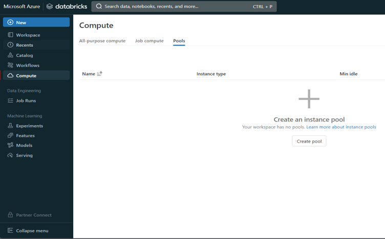
Figure 4 – Create instance pool-i

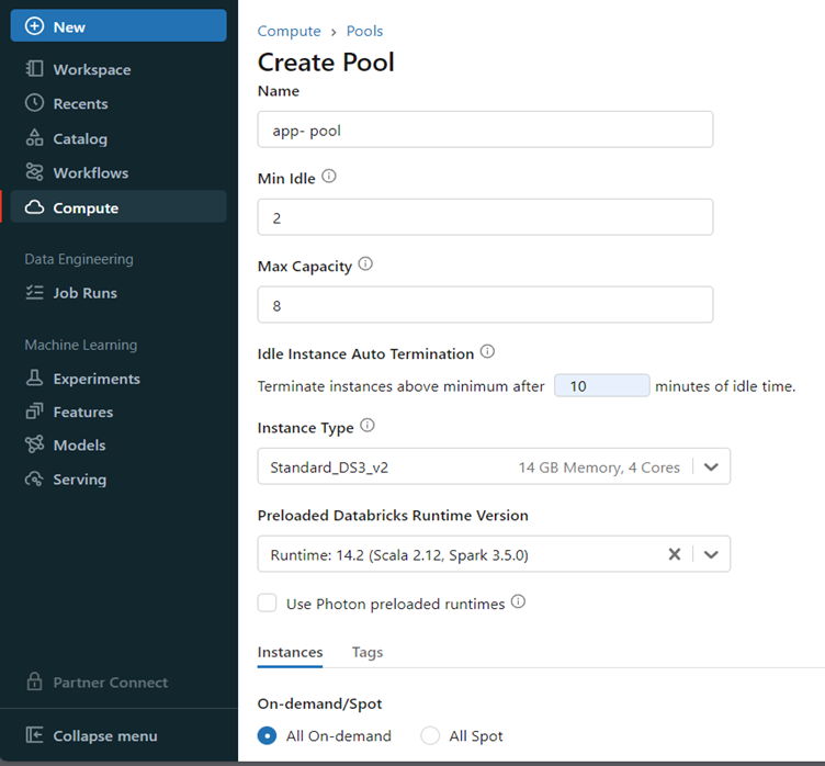
Figure 5 – Create instance pool-ii

4. Cluster optimisation for ADF parallelism

A few configuration adjustments are required for Azure Databricks clusters to function seamlessly with Azure Data Factory (ADF) and accelerate task completion. Initially, make sure the size of your Databricks cluster is appropriate for the task; it should correspond with the volume of data and your workload. To ensure that jobs may run concurrently without interruption, change the number of worker nodes.

Make sure that jobs may execute concurrently wherever feasible while configuring your ADF pipelines. This accelerates processes by utilising Databricks’ capacity to distribute work over several machines. Furthermore, arrange your data such that Databricks can handle it easily, and employ strategies that expedite data processing.

5. Autoscaling

You may set the cluster’s minimum and maximum worker count by turning on autoscaling. When autoscaling is enabled, the cluster may scale up or down based on the load. Databricks then determines the right number of workers needed to complete the task. The cluster cannot be started or stopped by users, but the initial on-demand instances are immediately ready. To handle the workload, autoscaling automatically supplies extra nodes (mainly Spot instances) if the user query demands more capacity.

This approach keeps the overall cost down by:

• Using a shared cluster model
• Using a mix of on-demand and spot instances
• Using autoscaling to avoid paying for underutilised

This presents significant advantages:

• Workloads can run faster compared to a constant-sized under-provisioned cluster
• Autoscaling clusters can reduce overall costs compared to a statically sized cluster.

How autoscaling behaves

Autoscaling behaves differently depending on whether it is optimised or standard and whether applied to an interactive or a job cluster.

Databricks offers two types of cluster node autoscaling: optimised and standard.

Optimised

1. Scales in two stages from minimum to maximum.
2. By examining the shuffle file status, it is possible to scale down even when the cluster is not idle.
3. Based on a fraction of active nodes, it scales down.
4. Scales down job clusters if they have not been used for the last 40 seconds.
5. Scales down interactive clusters if they have not been used over the last 150 seconds.

Standard

1. Adds four nodes first. After that, it scales up exponentially, however, it can take a while to reach the maximum.
2. Only shuts off once the cluster has been inactive for the last ten minutes and is dormant.
3. Takes one node and scales down exponentially from there.

6. Cost Management

To effectively optimise Databricks costs, you should understand the platform’s pricing model and the cost components that make up a Databricks environment.

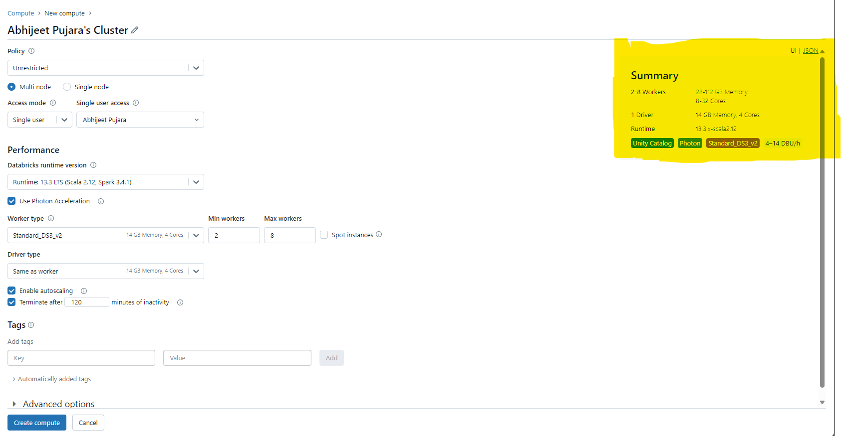
Figure 6 – Cost management of multi-node cluster

The cost of Databricks is determined by a consumption model that bills you for the resources required to complete your tasks. These resources consist of I/O, memory, and computers. Databricks units (DBUs), a measurement of the total number of resources consumed per second, are used to quantify each resource. You use these DBUs to figure out how much it costs to operate your workloads in Databricks. It may be difficult to determine how much it will cost to operate a Databricks environment since so many variables need to be taken into consideration. These include the size of the cluster, the kind of workload, the subscription plan tier, and—most importantly—the cloud platform that the environment is housed on.

The DBU rate of the cluster, which changes based on the subscription plan tier and cloud provider, is the key to figuring out how much a Databricks setup would cost. Aside from that, you also need to account for the sort of workload (automated job, all-purpose compute, delta live tables, SQL compute, or serverless compute) that produced the designated DBU.

DBU calculators can be used to estimate the expenses associated with running individual workloads and to determine the total cost of operating your Databricks infrastructure.

Conclusion

We looked at the nuances of setting up clusters with Azure Databricks in this article. We broke down single- and multi-node clusters to comprehend their functions, benefits, and drawbacks.

The main conclusions are as follows:

Single-node clusters: Perfect for light workloads, testing, and development. simplicity and economy of cost. restricted capability for parallelism and resources.

Multi-node clusters: Performance and scalability for heavy production workloads. Worker nodes divide up the work of processing. The driver node coordinates the execution.

Remember, cluster configuration directly impacts performance, cost, and user experience. Choose wisely based on your workload requirements.

Thank you for joining us on this journey through Azure Databricks clusters. Feel free to explore further and experiment with different configurations.

Happy Databricking!