Databricks – Cluster Sizing

Introduction

Setting up Clusters in Databricks presents you with a wrath of different options. Which cluster mode should I use? What driver type should I select? How many worker nodes should I be using? In this blog I will try to answer those questions and to give a little insight into how to setup a cluster which exactly meets your needs to allow you to save money and produce low running times. To do this I will first of all describe and explain the different options available, then we shall go through some experiments, before finally drawing some conclusions to give you a deeper understanding of how to effectively setup your cluster.

Cluster Types

Databricks has two different types of clusters: Interactive and Job. You can see these when you navigate to the Clusters homepage, all clusters are grouped under either Interactive or Job. When to use each one depends on your specific scenario.

Interactive clusters are used to analyse data with notebooks, thus give you much more visibility and control. This should be used in the development phase of a project.

Job clusters are used to run automated workloads using the UI or API. Jobs can be used to schedule Notebooks, they are recommended to be used in Production for most projects and that a new cluster is created for each run of each job.

For the experiments we will go through in this blog we will use existing predefined interactive clusters so that we can fairly assess the performance of each configuration as opposed to start-up time.

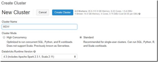
Cluster Modes

When creating a cluster, you will notice that there are two types of cluster modes. Standard is the default and can be used with Python, R, Scala and SQL. The other cluster mode option is high concurrency. High concurrency provides resource utilisation, isolation for each notebook by creating a new environment for each one, security and sharing by multiple concurrently active users. Sharing is accomplished by pre-empting tasks to enforce fair sharing between different users. Pre-emption can be altered in a variety of different ways. To enable, you must be running Spark 2.2 above and add the following coloured underline lines to Spark Config, displayed in the image below. It should be noted high concurrency does not support Scala.

Enabled – Self-explanatory, required to enable pre-emption.

Threshold – Fair share fraction guaranteed. 1.0 will aggressively attempt to guarantee perfect sharing. 0.0 disables pre-emption. 0.5 is the default, at worse the user will get half of their fair share.

Timeout – The amount of time that a user is starved before pre-emption starts. A lower value will cause more interactive response times, at the expense of cluster efficiency. Recommended to be between 1-100 seconds.

Interval – How often the scheduler will check for pre-emption. This should be less than the timeout above.

Driver Node and Worker Nodes

Cluster nodes have a single driver node and multiple worker nodes. The driver and worker nodes can have different instance types, but by default they are the same. A driver node runs the main function and executes various parallel operations on the worker nodes. The worker nodes read and write from and to the data sources.

When creating a cluster, you can either specify an exact number of workers required for the cluster or specify a minimum and maximum range and allow the number of workers to automatically be scaled. When auto scaling is enabled the number of total workers will sit between the min and max. If a cluster has pending tasks it scales up, once there are no pending tasks it scales back down again. This all happens whilst a load is running.

Pricing

If you’re going to be playing around with clusters, then it’s important you understand how the pricing works. Databricks uses something called Databricks Unit (DBU), which is a unit of processing capability per hour. Based upon different tiers, more information can be found here.You will be charged for your driver node and each worker node per hour.

You can find out much more about pricing Databricks clusters by going to my colleague’s blog, which can be found here.

Experiment

For the experiments I wanted to use a medium and big dataset to make it a fair test. I started with the People10M dataset, with the intention of this being the larger dataset. I created some basic ETL to put it through its paces, so we could effectively compare different configurations. The ETL does the following: read in the data, pivot on the decade of birth, convert the salary to GBP and calculate the average, grouped by the gender. The People10M dataset wasn’t large enough for my liking, the ETL still ran in under 15 seconds. Therefore, I created a for loop to union the dataset to itself 4 times. Taking us from 10 million rows to 160 million rows. The code used can be found below:

# Import relevant functions.

import datetime

from pyspark.sql.functions import year, floor

 

# Read in the People10m table.

people = spark.sql(“select * from clusters.people10m ORDER BY ssn”)

 

# Explode the dataset.

for i in xrange(0,4):

people = people.union(people)

 

# Get decade from birthDate and convert salary to GBP.

people = people.withColumn(‘decade’, floor(year(“birthDate”)/10)*10).withColumn(‘salaryGBP’, floor(people.salary.cast(“float”) * 0.753321205))

 

# Pivot the decade of birth and sum the salary whilst applying a currency conversion.

people = people.groupBy(“gender”).pivot(“decade”).sum(“salaryGBP”).show()

To push it through its paces further and to test parallelism I used threading to run the above ETL 5 times, this brought the running time to over 5 minutes, perfect! The following code was used to carry out orchestration:

from multiprocessing.pool import ThreadPool

pool = ThreadPool(10)

pool.map(

     lambda path: dbutils.notebook.run(

          “/Users/mdw@adatis.co.uk/Cluster Sizing/PeopleETL160M”,

timeout_seconds = 1200),

     [“”,“”,“”,“”,“”]

)

To be able to test the different options available to us I created 5 different cluster configurations. For each of them the Databricks runtime version was 4.3 (includes Apache Spark 2.3.1, Scala 2.11) and Python v2.

Default – This was the default cluster configuration at the time of writing, which is a worker type of Standard_DS3_v2 (14 GB memory, 4 cores), driver node the same as the workers and autoscaling enabled with a range of 2 to 8. Total available is 112 GB memory and 32 cores.

Auto scale (large range) – This is identical to the default but with autoscaling range of 2 to 14. Therefore total available is 182 GB memory and 56 cores. I included this to try and understand just how effective the autoscaling is.

Static (few powerful workers) – The worker type is Standard_DS5_v2 (56 GB memory, 16 cores), driver node the same as the workers and just 2 worker nodes. Total available is 112 GB memory and 32 cores.

Static (many workers new) – The same as the default, except there are 8 workers. Total available is 112 GB memory and 32 cores, which is identical to the Static (few powerful workers) configuration above. Therefore, will allow us to understand if few powerful workers or many weaker workers is more effective.

High Concurrency – A cluster mode of ‘High Concurrency’ is selected, unlike all the others which are ‘Standard’. This results in a worker type of Standard_DS13_v2 (56 GB memory, 8 cores), driver node is the same as the workers and autoscaling enabled with a range of 2 to 8. Total available is 448 GB memory and 64 cores. This cluster also has all of the Spark Config attributes specified earlier in the blog. Here we are trying to understand when to use High Concurrency instead of Standard cluster mode.

The results can be seen below, measured in seconds, a new row for each different configuration described above and I did three different runs and calculated the average and standard deviation, the rank is based upon the average. Run 1 was always done in the morning, Run 2 in the afternoon and Run 3 in the evening, this was to try and make the tests fair and reduce the effects of other clusters running at the same time.

Before we move onto the conclusions, I want to make one important point, different cluster configurations work better or worse depending on the dataset size, so don’t discredit the smaller dataset, when you are working with smaller datasets you can’t apply what you know about the larger datasets.

Comparing the default to the auto scale (large range) shows that when using a large dataset allowing for more worker nodes really does make a positive difference. With just 1 million rows the difference is negligible, but with 160 million on average it is 65% quicker.

Comparing the two static configurations: few powerful worker nodes versus many less powerful worker nodes yielded some interesting results. Remember, both have identical memory and cores. With the small data set, few powerful worker nodes resulted in quicker times, the quickest of all configurations in fact. When looking at the larger dataset the opposite is true, having more, less powerful workers is quicker. Whilst this is a fair observation to make, it should be noted that the static configurations do have an advantage with these relatively short loading times as the autoscaling does take time.

The final observation I’d like to make is High Concurrency configuration, it is the only configuration to perform quicker for the larger dataset. By quite a significant difference it is the slowest with the smaller dataset. With the largest dataset it is the second quickest, only losing out, I suspect, to the autoscaling. High concurrency isolates each notebook, thus enforcing true parallelism. Why the large dataset performs quicker than the smaller dataset requires further investigation and experiments, but it certainly is useful to know that with large datasets where time of execution is important that High Concurrency can make a good positive impact.

To conclude, I’d like to point out the default configuration is almost the slowest in both dataset sizes, hence it is worth spending time contemplating which cluster configurations could impact your solution, because choosing the correct ones will make runtimes significantly quicker.