As I see it, Graph Theory is the dark horse of Business Intelligence. It comes in many names and variations: Social Network Analysis, Network Science or Network Theory, but they all have the same algorithms and principles. A common misconception is that graph theory only applies to communication data such as online or traditional social networks or a network of computers and routers. This blog aims to show you how Graph Theory algorithms can uncover hidden insights in a range of business data. I *promise* to keep this light on mathematics and heavy on business value.
Let’s first get stuck in with some terminology and network graphs.
Basic Terminology
As with any mathematical study, Graph Theory comes with a fair handful of jargon:
- Node(s) – Sometimes called Vertex/Vertices, Nodes are one of two of the most important properties of a network graph. They are simply an entity on the graphs that represents an intersection/connection. This could be a person, location, product, an idea etc. Visually, it is usually represented as a circle.
- Edge(s) – Sometimes called Tie(s) or Link(s), Edges are the second most fundamental property of a network graph, an edge is the link between two connections. Visually, it is usually represented as a line connecting the nodes.
- Weight – A weight is a numerical attribute of an edge that should be considered when calculating certain graph theory metrics. An example would be when calculating the shortest route through a geographical network, the distance measure between each location should be considered.
- Neighbour(s) –Neighbours are 2 nodes connected by an edge.
- Path – A path is a route (of edges) between 2 or more nodes.
Network Graphs
Below are examples of network graphs:
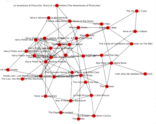
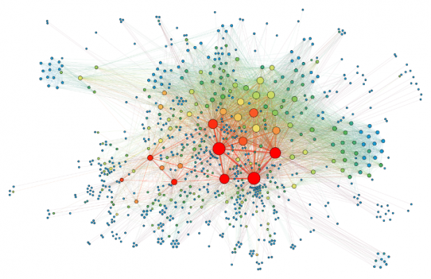
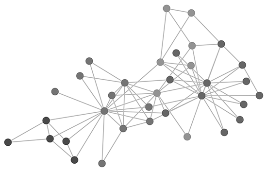
The network graph on the left is a network of 40 books as the nodes and co-purchasing links as the edges which I visualised in a previous blog. The network graph on the right is taken from a research article by Martin Grandjean.
Despite the differences in colour and size, these are both examples of plain vanilla network graphs. Martin Grandjean’s graph on the right is also great visual example of two popular graph theory metrics: the size of the nodes is dictated by their Degree Centrality and the colour is dictated by their Betweenness Centrality. These two metrics will be discussed later in the article but it’s great to know that the results of graph theory algorithms can also be visualised on a network graph.
Below are two more (slightly fancier) network graphs:
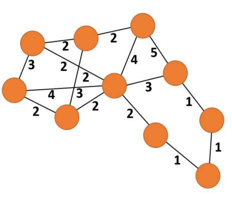
The graph in orange (left) is an example of a weighted graph. This is a network where the edges among nodes have weights assigned to them. When visualised, weights associated with an edge can be represented by a number, like in the example above, or by the thickness of the line.
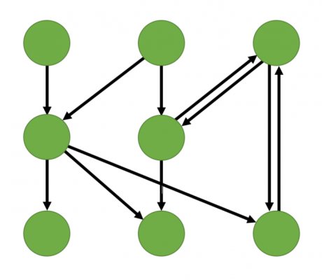
The graph in green (right) is an example of a directed graph. This is a network where the edges among nodes have a direction assigned to them. Directed graphs will have an arrow as opposed to a line to represent the edge and direction. Some algorithms will take the direction into consideration when calculating metrics.
It is possible, and quite popular, for a graph to be both weighted and directed.
Example of Network Graphs in Business Intelligence
One reason graph theory usually is often overlooked when organisations build their business intelligence roadmap is that the strategists responsible don’t see any examples of network graphs that apply to their own data. Network graphs can be built from any data that has relationships, not just social networks or computer networks. Here are some examples:
- All the flights to and from airports can be organized as a graph. In this case, the airports are the nodes and the flights the edges between the nodes.
- The accounts of a bank with all the money transfers form a graph.
- All deliveries between addresses worldwide can be organized as a network graph.
- A visitor’s journey on an organization’s website can also form a graph, where webpages form the nodes and the visitor’s movements become the relationships.
- In retail, products can be the nodes linked together by co-purchases to form a network graph.
As you can see, network graphs are a fantastic way to represent and visualise the relationships between entities. But this isn’t their only purpose. Network graphs are usually built to provide a unique data structure to perform calculations upon.
This brings us to my favourite subject…
Graph Theory Algorithms!
Centrality
The centrality metric comes in many flavours with the most popular including Degree, Betweenness and Closeness. These are used to calculate the importance of a particular node and each type of centrality applies to different situations depending on the context.
Degree centrality is by far the simplest calculation. It is a count of how many edges are connected to each node. A node with a high degree centrality, which is a node with lots of edges, is generally considered a highly active node. If the network graph represented a network of flights between airports, the airport with the highest degree centrality would be the busiest airport. (Centrality can be further granulated by splitting it into 2 values, the in-degree and out-degree, in directed graphs. These values can determine whether a node is prominent, with lots of other nodes reaching towards it, or influential, with the node itself reaching out to many other nodes.)
Betweenness centrality is a measurement of how often a particular node lies on a shortest path between two other nodes. A high betweenness centrality would suggest that the removal of that node would increase the distance between a lot of other nodes. Again, if the network graph represented a network of flights between airports, all airports with a high betweenness centrality would likely make excellent layover/ connecting airports because they lie on the shortest route between two indirectly connected airports.
Closeness centrality is a measure of proximity of a node to other nodes. A node with a high closeness can broadcast information quickly and in social networks a person that has a high closeness centrality is an important person. In the context of a network of flights, the airports with high closeness centralities would most likely have lots of quick small flights outbound and inbound. Closeness centrality has been used in studies to recognise individuals in positions to control information and resources within an organisation, used as a metric for estimating arrival times of package deliveries and to calculate the importance of certain words and phrases in documents using graph-based key-phrase extraction.
As a general rule, centrality metrics will be positively correlated. By this I mean that nodes with high degree centrality scores will commonly have high betweenness and closeness centrality scores. However, this isn’t always the case. When the above centrality metrics appear to conflict with each other, there is likely something really interesting about the position of the node in the network. Refer to the table below to see how this plays out:
| Low Degree Centrality | Low Betweenness Centrality | Low Closeness Centrality | |
| High Degree Centrality | The node will have many connections, but they will mainly be nodes with few connections making it inconsequential for the networks flow. | Node is likely embedded in a cluster far from the rest of the network. | |
| High Betweenness Centrality | The node will have few connections but the ones it does have will be important for the networks flow. | This would be an unlikely scenario but would occur when the node lays on the majority of the paths that connect otherwise disconnected nodes to central nodes. | |
| High Closeness Centrality | A highly central and influential node which doesn’t have many directly connected nodes. | You would likely find the network is very dense. This node will be near to many other nodes, but so will a lot of others in the network. |
PageRank
PageRank (PR) is another centrality metric, but I thought it was worthy of its own section.
PageRank’s claim to fame is that it was first algorithm used by Google to rank websites in their search engine results. The PageRank algorithm is based on the premise that the importance of a node depends on the importance of its neighbours, which in turn depend on the importance of their neighbours, and so on.
As with all graph theory algorithms, PageRank can be applied to network graphs in any context or domain – not just to search engines. For example, in neuroscience, the PageRank of a neuron in a neural network has been found to correlate with its relative firing rate and, in ecology, PageRank can be used to determine species that are essential to the continuing health of the environment.
Twitter uses this algorithm on a graph of users which contains shared interests and common connection to present users with recommendations of other accounts to follow.
Assortativity
The assortativity algorithm is another really cool concept. It measures the preference for a network’s nodes to connect to others that are similar in some way.
Online social networks such as Twitter or Facebook provide a heap of proof of assortativity uncovering hidden insights in big data. For example: One study uncovered that twitter users who tweeted far from their expected location (ie when travelling away from home) were much more likely to create posts containing positive language. Another study uncovered that those who post positive tweets were more likely to interact with others with a high happiness score, alternatively those who were unhappy and post negative tweets were more likely to be connected to others of a similar poor well-being.
The resilience of a network is often dictated by the assortativity coefficient which makes the properties of assortativity very useful in fields such as epidemiology, since they can help understand the spread of disease or cures.
Other Simple (but no less insightful) Graph Metrics
- Density: A ratio of total edges present in a network to total edges possible in a network.
- Cliques: A clique is a group of nodes which are all connected to one another. One graph can contain hundreds, even thousands, of sub-graphs that can be defined as cliques.
- Bridges: This is the name for an edge which will disconnect a graph if it were to be removed.
- Clustering Coefficient: This metric is a measure for ‘how much’ nodes in a graph tend to cluster together.
Graph Theory in Business Intelligence
The application of all the above algorithms has never been simpler. Programming libraries and tools have been built to take all the complexity of graph theory and abstract this behind GUIs and commands. My favourites include NetworkX (this python library is intuitive and powerful) and Gephi (a network visualisation tool perfect for those exploring graph theory with no programming background). Graph databases such as Neo4j, Gremlin and CosmosDB are making graph theory easier to productionise.
Graph Theory as a theme for data analytics and data science isn’t a new concept – it is used in studies into online social networks, it forms a significant role in Artificial Neural Networks and has also gained recognition as a useful framework in which to consider the human brain in terms of its structure and function but in the realm of Business Intelligence, graph theory is underestimated.
PS. I surprisingly pulled through on my promise to be light on the mathematics – not a single equation in sight!
Introduction to Data Wrangler in Microsoft Fabric
What is Data Wrangler? A key selling point of Microsoft Fabric is the Data Science
Jul
Autogen Power BI Model in Tabular Editor
In the realm of business intelligence, Power BI has emerged as a powerful tool for
Jul
Microsoft Healthcare Accelerator for Fabric
Microsoft released the Healthcare Data Solutions in Microsoft Fabric in Q1 2024. It was introduced
Jul
Unlock the Power of Colour: Make Your Power BI Reports Pop
Colour is a powerful visual tool that can enhance the appeal and readability of your
Jul
Python vs. PySpark: Navigating Data Analytics in Databricks – Part 2
Part 2: Exploring Advanced Functionalities in Databricks Welcome back to our Databricks journey! In this
May
GPT-4 with Vision vs Custom Vision in Anomaly Detection
Businesses today are generating data at an unprecedented rate. Automated processing of data is essential
May
Exploring DALL·E Capabilities
What is DALL·E? DALL·E is text-to-image generation system developed by OpenAI using deep learning methodologies.
May
Using Copilot Studio to Develop a HR Policy Bot
The next addition to Microsoft’s generative AI and large language model tools is Microsoft Copilot
Apr