Timespan Fact Table

This blog focuses on a fact table primarily used for storing semi-additive measures such as balance amounts. Other examples include inventory levels and room temperatures which are non-additive across the date dimension. As per Kimball,

“Semi-additive measures can be summed [..] across all dimensions except time”

In these cases, the measure may be aggregated across dates by averaging over the number of periods, e.g., average daily inventory levels. Measures can also be aggregated across dates by taking the maximum/minimum for the time interval.

More specifically, this blog focuses on an alternative approach to providing end users with the ability to do point-in-time analysis, so-called trend analysis.

Simple Illustration

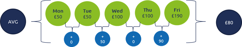
The following is an example of the account balance for customer X. The account transactions are tracked throughout the week, starting on Monday with periods of no activity on Monday & Wednesday. On Friday, we can’t merely add up the daily balances during the week and declare that the ending balance is £490. The most helpful way to combine account balances across dates is to average them, which results in an average daily balance of £98.

Often a Fact Table will store transaction-level data for a given day using a truncate and reload pattern. The above illustration would result in at most 1 row within said Fact Table.

However, end users often require history tracking within a fact table to cater for the following reporting date scenarios.

• As of (reporting date)
• From a date to a date
• Changes between days

Accepted Approach: Periodic Snapshot

The accepted approach is through a Periodic Snapshot. Kimball states,

“A row in a periodic Snapshot fact table summarizes many measurement events occurring over a standard period, such as a day, a week, or a month. The grain is the period, not the individual transaction [..].”

All the rows for a given time interval will be inserted into the periodic snapshot fact table with a Snapshot Date as a timestamp, allowing for point-in-time reporting. The table can grow considerably over time, depending on data volumes and time intervals.

Simple Illustration: Periodic Snapshot

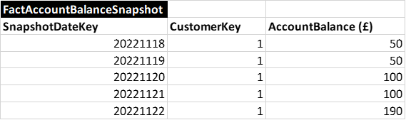
Unlike the Transactional Fact Table, which stores, at most, 1 row for customer X in the above scenario. This Periodic Snapshot runs daily snapshots resulting in 5 rows (below). The SnapshotDateKey is the mechanism through which users can perform trend analysis.

Alternative Approach: Timespan Fact Table

As per Kimball,

“In isolated cases, it is useful to add a row effective date, row expiration date, and current row indicator to the fact table, much like you do with type 2 slowly changing dimensions, to capture a timespan when the fact row was effective.”

This approach can be used to address slowly changing balances. As a result of daily snapshots on the above FactAccountBalanceSnaphot table, we end up loading identical rows with each Snapshot (Row 2 & 4).

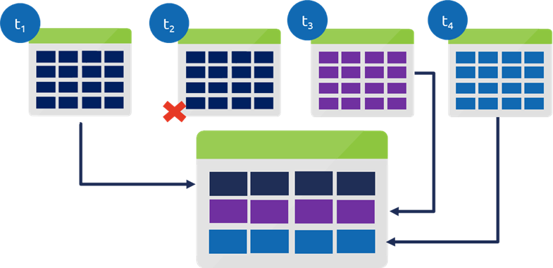
With a Timespan Fact Table, we would only insert a new record where a change occurred. Instead of simply inserting a new record into the table, this pattern requires a lookup against the table before evaluating whether to insert a new record.

Whilst this approach results in a lot less redundant data than a periodic snapshot, it does, however, require more compute resources during the ETL process.

Simple Illustration: Timespan Fact Table

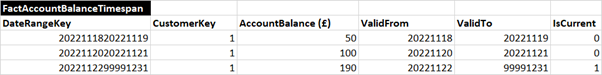
Going back to our scenario, we’ve already seen that the Transactional Fact Table stores, at most, 1 row for customer X. The Periodic Snapshot stores five rows. The Timespan will store three records as the account balance only changed twice during the week.

Timespan Fact Table: Bridge Table

The records in the Fact table need to be filtered by date to perform the point-in-time analysis. We need a way to associate the fact table with the date dimension, however we only have a date range, so we need a bridge table to associate both tables.

We need the bridge table to take all the unique data ranges within the fact table and explode them to get all the dates within each range.

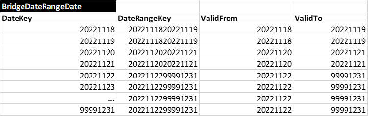
We can then join to the Date Dimension using the DateKey and join to the Timespan Fact using the DateRangeKey.

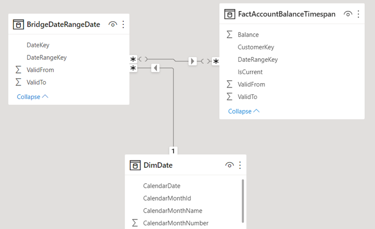
The relationship between the Bridge table and the Timespan will be many: many as there will be similar data ranges across customers in the Timespan table. By design, the bridge table repeats the data range for all the dates in between. A many: many relationship is unavoidable. This shouldn’t be problematic for this case so long as the filter direction is set up so that DimDate filters the Bridge table, which in turn filters the Timespan fact table.

Final Thoughts

Correctly configured, this approach allows report designers to empower end users to self-serve with the added flexibility of quickly getting a current and historical view of the data. If you’re interested in enabling your team to self-serve business intelligence within Power BI, we have a range of services that might be of interest.

The following section contains an assessment of the pros and cons of this approach.

Benefits

• One fact table is required, whereas Periodic Snapshot is at least 2 (Transactional fact table and the Period Snapshot fact table)
• No need to build a snapshot scheduler; therefore, orchestration is more straightforward than a Periodic snapshot.
• The benefit of daily Snapshots without snapshotting every day gives the BI team tremendous flexibility without the storage demands necessitated by daily snapshots.

Concerns

• Longer ETL, especially as data grows over time. Periodic Snapshot is just an insert, whereas Timespan requires a lookup before an insert. You will need to consider your ETL window.
• Many: many join between the bridge table and the Timespan fact table. As previously stated, this is unavoidable; however, it should be harmless if the filter directions have been set up correctly.

Acknowledgements

Although the inspiration for the blog stemmed from a client requirement, I credit my understanding of the approach to Davide Mauri, who’s SQL bits presentation is proving timeless ten years on.

Additional Reading

• Blog on the alternative approach discussed above
• Blog on the accepted approach also discussed above