A multi-valued attribute in data warehousing terms is a dimension attribute that has more than 1 value for a particular dimension member. Rather than focus too much on the warehouse technique in question Vincent Rainardi’s blog post provides a very good technically agnostic explanation far better than I could.
When we come to model this in SSAS we can consider each of solutions presented by Vincent:
- Lower the grain of the dimension
- Put the attribute in another dimension, linked directly to the fact table
- Use a fact table (bridge table) to link the 2 dimensions
- Have several columns in the dim for that attribute
- Put the attribute in a snow-flaked sub dimension
- Keep in one column using columns or pipes
Option 6 isn’t very practical or elegant for SSAS since it implies that you’d have front end that has the intelligence to separate out the delimited values and deal with the facts appropriately. This is not very practical considering how tools like Excel and Reporting Services access the Unified Dimensional Model (UDM).
Option 4 again isn’t very SSAS friendly regarding presentation and can get out of hand very quickly. In scenarios where multivalued attributes occur it can be very prevalent across the business, often where products are classified many different ways, for example Movies. Creating columns for every value for every multi-valued attribute can become a bit of a mare, also it’s not a very dynamic solution.
Option 2, placing the attribute in another dimension whilst it will work isn’t very elegant from a user perspective because of the way SSAS exposes dimensions and attributes. Conceptually from a user navigation and analysis perspective they are attributes of the same dimension and thus should be organised as such without having to query across the fact table to get the results you want. Once you’ve separated the attributes into separate dimensions you cannot build hierarchies that provide intuitive guidance to how users should explore and report the data. Also, it gets even trickier since you have to lower the grain of the fact table to avoid double counting which means allocation! Allocation can be a tricky, sluggish and ETL labouring solution. I do acknowledge however that pushing back logic to the ETL layer can do wonders for reporting query response times.
To get the desired output in SSAS I’m going to make use of a mixture of options 1, 2 and 3 with some slight but important differences to how Vincent has stated them. I will lower the grain of the dimension logically and not physically. I’ll put the attributes in a second dimension but link indirectly to fact table through the bridge table presented in option 3. I’ll also use some SSAS configuration in order to present all the attributes in what appears to be a single physical dimension linked directly to the fact table for the user.
The Solution
So our aim:
- Accommodate multi-valued attributes in a single dimension exposed to the user
- Avoid complex allocation procedures to lower the grain of the fact table
- Accommodate many-to-many relationships between multi-valued attributes without double counting the fact
For our example we’ll consider a great passion of mine Movies! Consider a basic additive measure with 2 dimensions:
Measure Viewings
Dimension Movie
Dimension Date
Conceptually the Movie dimension has the following attributes associated with it:
- Name (Single Value)
- Genre (Multi-Value)
- Theme (Multi-Value)
- Language (Multi-Value)
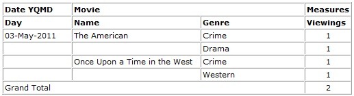
So if we consider 1 viewing of “The American” directed by Aton Corbijn and 1 viewing of “Once Upon a Time in the West” directed by Sergio Leone, we want the data to appear as follows:

Table 1: Movie Report by Name
However we break it out by the attributes the total is always 2 since there has only been 2 viewings i.e. we’re not double counting. If we were to report the Movie dimension by Genre alone then the results would be as follows since 2 viewings count towards Crime and 1 viewing counts towards Drama and Western, however the total viewings is still only 2.
 Table 2: Movie Report by Genre |
|

The meta data in Figure 1 shows a basic Date dimension and the Viewing measure. It also shows the Movie dimension containing the Movie (name) and the multi-valued attributes Genre, Language and Theme all nicely organised into the movie dimension. If desired we could provide more structure to the Movie dimension by creating hierarchies since they all belong to the same dimension.
The Pattern
Being familiar with how SSAS models I tend to think of this first and foremost as a fact table grain problem rather than dimensional problem. Essentially we need to lower the grain of the fact table to avoid double counting across the multi-valued attributes. If we’re not going to allocate down the measures we can do this using bridge table in SSAS and then use a bit of design trickery to hide the intermediate dimension and expose all the attributes in the outer dimension for the users to browse.
Relation Model
Figure 2 shows the structure of the source relational database:

Figure 2: Relational Database Model
The dimensions are highlighted blue and the fact / bridge tables are grey. Over to the right hand side we see the basic star schema which is the FactViewings with the 2 dimensions DimMovieName and DimDate containing single value attributes. Over to the left hand side we see that DimMovieName is joined to a DimMovieMVAJunk through a bridge table called BridgeMovieMVAJunk.
The DimMoveMVAJunk contains a Cartesian product of all the possible multi-valued attributes. We chose to use a junk dimension because in our particular dimension the data volumes aren’t particularly that scary and we don’t have to concern ourselves too much about the actual relationships between the multi-valued attributes that exist or could exist in our data. Any relationships that exist today may be different tomorrow so we’ll just treat all the multi-valued attributes as many to many. If we know this then we can pre-populate the junk dimension with all the combinations we could possible encounter and give it a surrogate key.
The BridgeMovieMVAJunk maps the multi-value attributes to single value attribute in DimMovieName. We use a bridge table since we can assign more than one value of an attribute to 1 particular Movie. We cannot combine MovieName and the other attributes together and bind them to the FactViewings table because the grain key of the fact table is MovieKey. If we combine all the attributes the MovieKey of the DimMovieName will no longer be the grain and SSAS will not report the correct values against the attributes and totals. The bridge table we just populate with the actual relationships that exist between DimMovieName and all the other attributes. The bridge table is effectively a fact less fact table and we can use the same fast loading techniques on a bridge table that we can use on a regular fact table i.e. it’s easy it manage and load.
Also in the database we’ll use the following logic to create the view that will feed the Movie dimension in the cube that the users will use and see.
CREATE VIEW [DimMovie]
AS
SELECT
m.[MovieKey],
j.[MovieMVAJunkKey],
m.[MovieName],
j.[Genre],
j.[Language],
j.[Theme]
FROM DimMovieName m
INNER JOIN BridgeMovieMVAJunk b ON m.MovieKey = b. MovieKey
INNER JOIN DimMovieMVAJunk j ON j.MovieMVAJunkKey = b.MovieMVAJunkKey
Please note the grain of this dimension is now a component key of the single value attributes and the multi value attributes. Also ensure the database is adequately tuned for the execution of this statement otherwise (depending on data volumes) you might find it takes a while for your Movie dimension to process. You could also do this in the Data Source View (DSV) of the UDM but I’m not a fan of placing logic in the DSV unless there is real cause to do so.
UDM
Figure 3 shows the structure of the SSAS DSV.

Figure 3: SSAS Data Source View
The SSAS DSV is almost identical to the relation model except we’ve used the view DimMovie that combines all the movie attributes together and joined it to the bridge using the component key i.e. we’ve tagged the single value attributes onto the multi-valued attributes to get our complete dimension.
Figure 4 shows the cube structure in SSAS where we’ve created 2 measure groups and 3 dimensions.

Figure 4: Cube Structure
We have a fact table containing the core measures, which in our case [FactViewings] has been added as a measure group called [Viewings]. We have bridge table called [BridgeMovieMVAJunk] that is added in as a measure group called [BridgeMovieAttributes] but either hide the default count measure or delete it completely so that the users are unaware that this measure group exists.
The [System Movie] dimension is created from the [DimMovieName] table and as the name implies is for utility purposes and will be hidden using the visible property. This dimension simply contains the grain key of the single-value attributes and is used as an intermediate dimension to bind to [FactViewings]. The [Movie] dimension is created from the [DimMovie] view dimension and contains all the movie attributes and binds to the [BridgeMovieMVAJunk] using a component key.
Figure 5 shows the dimensionality.

Figure 5: Cube Dimensionality
The final setup for the cube is to ensure the dimensionality is configured correctly. Here we see [System Movie] sits across both measure groups using a regular relationship, remember that [System Movie] and [Bridge Movie Attributes] are both hidden. The [Movie] dimension is bound to [Bridge Movie Attributes] using a regular relationship, when creating this relationship you must ensure the relationship is bound using the full component key i.e. [MovieKey] and [MovieMVAJunkKey]. The [Movie] dimension is then bound to the core measure group [Viewings] using a many to many relationship.When processed you should end up with the meta-data presented in figure1. All fairly straightforward!
The Results
Ok, so now we have a structure that we think will do the job. All is left to do is stick in some data and see if it works. I’ve set up the data in my table with the following movie classifications:

Table 3: Movie Classifications
I’ve also set up the data with the following viewings:

Table 4: Movie Viewings
Having loaded the data and processed the cube I’ve pulled out the data in Excel which can be seen in Figure 6 and figure 7.

Figure 6: Reporting Against a Single Attribute
In figure 6 we can see the meta-data nicely organised with the single and multi-value attributes all available together under the single [Movie] dimension. In Movie Viewings report notice that summing the figures correctly matches the total value of 21. Below that report is the Genre Viewings report, notice here that if we manually sum up the viewing figures we’ll get 49 which is not correct since we’ll be double counting viewings where a movie exists in more than one Genre. The cube grand total correctly shows 21 and does not double count the viewings because of the logic we have created to handle multi-valued attributes

Figure 7: Reporting Against Multiple Attributes
In figure 7 we can see how single and multi-value attributes work side by side in further detail. Notice that Genre totals are a sum of the viewings for Movies within the Genre. Also notice that Movies exist in more than one Genre and yet the Grand Total is still only 21 and that we are not double counting e.g. the viewings for ‘Very Bad Things’ count towards Thriller, Crime and Comedy.
I’ve included other multi-value attributes in the design pattern just to show how it can be done. I’ve only played with one multi-valued attribute here in so that I don’t end writing the world’s longest blog post! So by all means knock up cube and have a play and you should see that all the attributes work nicely together.
Conclusion
We’ve successfully modelled multi-valued attributes into a single dimension within a cube whilst handling the issue of aggregating correctly by:
- Lowering the grain of the dimension to store all the multi-value attributes together in a junk dimension
- Creating a bridge table to map the multi-value attributes to the single value attributes
- Linking all the attributes in a single dimension to the fact table through the bridge table and single-value attribute dimension
We used the many to many dimension functionality of SSAS along with the customisation of some properties to bind the single and multi-value attributes onto the core fact whilst hiding the complexity involved from the user.
In terms of scalability and performance it’s going to really depend on your situation. We’ve pushed the logic into the cube structure and processing so it’s definitely going to be a lot better than using lots of complex MDX scoping which I’ve seen some solutions try to use. If the bridge table and junk dimension are quite large then you might need to keep an eye on processing performance since our Movie dimension is joining across those two tables plus the single value attribute dimension. The use of many to many SSAS relationships isn’t great for performance though it depends on the volumes, other complexities and any tuning you have performed on your cube. All in all it’s an elegant and simple design pattern that works well making the use of the cube structure without having to do lots of work in the warehouse to reduce the fact table grain.
Introduction to Data Wrangler in Microsoft Fabric
What is Data Wrangler? A key selling point of Microsoft Fabric is the Data Science
Jul
Autogen Power BI Model in Tabular Editor
In the realm of business intelligence, Power BI has emerged as a powerful tool for
Jul
Microsoft Healthcare Accelerator for Fabric
Microsoft released the Healthcare Data Solutions in Microsoft Fabric in Q1 2024. It was introduced
Jul
Unlock the Power of Colour: Make Your Power BI Reports Pop
Colour is a powerful visual tool that can enhance the appeal and readability of your
Jul
Python vs. PySpark: Navigating Data Analytics in Databricks – Part 2
Part 2: Exploring Advanced Functionalities in Databricks Welcome back to our Databricks journey! In this
May
GPT-4 with Vision vs Custom Vision in Anomaly Detection
Businesses today are generating data at an unprecedented rate. Automated processing of data is essential
May
Exploring DALL·E Capabilities
What is DALL·E? DALL·E is text-to-image generation system developed by OpenAI using deep learning methodologies.
May
Using Copilot Studio to Develop a HR Policy Bot
The next addition to Microsoft’s generative AI and large language model tools is Microsoft Copilot
Apr