An Ode to the Humble Decision Tree

When starting out in machine learning, the theoretical challenges associated with the field can seem unsurmountable, with scary names being fired left, right and centre. What on earth is a Hidden Markov Model? How does Principal Component Analysis affect my life? Why would anyone want to restrict a Boltzmann Machine? It feels like without quitting your job and spending the rest of your days studying niche statistical techniques, the deepest secrets of artificial intelligence will never be revealed.

While it is true there are techniques in machine learning that required advanced maths knowledge, some of the most widely used approaches make use of knowledge given to every child at secondary school. The line of best fit, drawn by many a student in Year 8 Chemistry, can also be known by its alter-ego, linear regression, and see applications all over machine learning. Neural networks, central to some of the most cutting-edge applications, are formed of simple mathematical models consisting of some addition and multiplication.

A personal favourite technique, and the subject of this blog, is the humble decision tree, taught in schools all over the country. This blog will take a high-level look at the theory around decision trees, an extension using random forests, and the real-world applications of these techniques.

Decision Trees

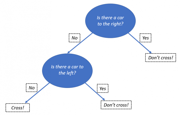
Decision trees are often used as a visual aid, in order to model a decision-making process. To illustrate the process, we can use an example of crossing the road. We start by looking to the right, and check for cars approaching. If there is a car, then we don’t cross the road. However, if there isn’t a car, then we can check for cars to the right. If there are no cars approaching, then we can progress to crossing the road.

As this technique is used for taking the data known about a situation, observing the data and then deciding on what course of action to take, it is easy to see how this could be used for making predictions. This allows us to take decision trees into the domain of machine learning. Whilst this article will not be going into the details of how computers form decision trees, a high-level view is that they take a measurement, called information gain, at each step that a decision is needed to split the data set. This step can be repeated until the data being used for training can be fully predicted by the decision tree.

Information gain is a measure in the change of entropy within the unpredicted data. Entropy, for those unfamiliar, is a measure of disorder within a system, sometimes called (dramatically) chaos. We wish to minimise the entropy in the data as it passes through the decision tree, which in layman’s terms mean we want the training data to be sorted into groups with same label or classification. By using an algorithm that maximises information gain at each step, effective decision trees can be formed without human input.

The technique produced allows for an easy to implement and highly interpretable model to perform classification, however one that often sees poor predictive performance on more complex applications. To resolve this, we can make use of an extension to decision trees using bagging and bootstrapping.

Random Forests

Say you want to buy a new car, but you don’t know the first thing about them. Cars are an expensive purchase, so you want to get some advice before the purchase. You ask your friend Carol, who is a coach driver, and she recommends a people carrier so you can fit more people in. You then ask Darren, who is obsessed with racing cars, and he recommends a car with a large engine so you can go faster. By asking more and more people, who have different expertise, and then taking the most popular answer, you should be able to find the best car for your needs.

The same intuition is used for creating random forests, where many decision trees will be consulted and the most popular/average prediction made will be used as the output for the model, similar to consulting a diverse selection of people before making a decision. In statistics, this is known as bagging. The ‘randomness’ of the group of decision trees is used to create diversity within the predictions made. In order to promote randomness, each decision tree will have access to a random subset of the training data, known as bootstrapping, and access to a random subset of the data’s features. The diversity of the decision trees created is analogous to the different people consulted having different experiences and interests, leading them to give different recommendations.

Although the intuition underlying random forests is simple, they have been used in a wide range of applications, from aircraft engine diagnoses through to detecting the risk of diabetic patients suffering blindness. They have even been used to predict the future prices of stocks, for those financially inclined. However, in the age of GDPR, the key issue affecting random forests is that the more decision trees within the forest, the predictions become more uninterpretable. This becomes problematic with respect to GDPR’s Article 15. Nevertheless, random forests are still a useful and versatile technique.

Conclusion

The aim of this blog post was not to try and prove that a strong foundation in maths is completely unneeded for machine learning, rather that one can get started with learning some of the core techniques and their applications without too much trouble. Further techniques that use mathematical principles taught at school include Naïve Bayes, making use of basic probability theory, and Bayesian Networks, an extension to the former.