Getting Started with PyTorch: A Deep Learning Tutorial

PyTorch is a deep learning framework created by the Artificial Intelligence Research Group at Facebook to build neural networks for machine learning projects. It isn’t brand new; PyTorch has been around since October 2016, almost exactly two years ago, but only now it is gaining the momentum it deserves. When used as an alternative to Keras, TensorFlow or NumPy, PyTorch shines in the following areas:

• It is very tightly integrated with native Python API’s which allows it to seamlessly interact with Python libraries such as NumPy, SciPy and Pandas.
• This also includes native debuggers so there is no need for a specialist debugger – Looking at you, TensorFlow…
• It supports both forward passes for prediction and back propagation using the Autograd library for training.

And most importantly:

• PyTorch builds dynamic computation graphs which can run code immediately with no separated build and run phases.
• This makes the neural networks much easier to extend, debug and maintain as you can edit your neural network during runtime or build your graph one step at a time.

** Note: If the basics of Deep Learning, Neural Networks and Back Propagation are alien to you or even if you fancy a little revision, I really recommend that you check out 3Blue1Brown’s awesome YouTube playlist covering the foundations of Neural Networks: https://www.youtube.com/playlist?list=PLZHQObOWTQDNU6R1_67000Dx_ZCJB-3pi **

In this tutorial I will introduce a basic deep neural network in PyTorch and explain the important steps along the way. Now, let’s get started!

Installation

The simplest and recommended way to install PyTorch is through a package management tool like Conda or Pip but it can be installed directly from source using the instructions found at: https://pytorch.org/

Install using Pip

Linux:

pip3 install torch torchvision

Mac:

pip3 install torch torchvision
# MacOS Binaries dont support CUDA, install from source if CUDA is needed

Windows:

pip3 install http://download.pytorch.org/whl/cu90/torch-0.4.1-cp37-cp37m-win_amd64.whl
pip3 install torchvision

Install using Conda

Linux:

conda install pytorch torchvision -c pytorch

Mac:

conda install pytorch torchvision -c pytorch
# MacOS Binaries dont support CUDA, install from source if CUDA is needed

Windows:

conda install pytorch -c pytorch
pip3 install torchvision

PyTorch can be installed on Azure Databricks as a Databricks PyPI library and comes preinstalled and configured on Azure Data Science Virtual Machines.

Dataset Selection

I originally found the dataset used in this tutorial in the UCI Machine Learning Repository. The dataset represents data on 11,000+ instances of phishing and non-phishing webpages which have 30 categorical attributes including PageRank, AbnormalURL, Google_Index and age_of_domain. The data also contained a label, 1 or -1 indicating if the webpage with a phishing webpage or not. The aim of this tutorial is to show how to use a deep neural network, so all data was cleansed before being split into two separate CSV files, train.csv and test.csv.

Simple Neural Network Design

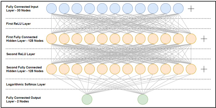
The neural network I will build consists of:

• 30 input nodes each representing a column of the dataset.
• These are passed through the first ReLU layer. Rectified Linear Units (ReLU) improve neural networks by speeding up training – all negative numbers are set to 0 and positive aren’t changed to speed up computations.
• Next is the first hidden layer consisting of 128 fully connected nodes.
• Then we have the second ReLU layer and second fully connected hidden layer which also consists of 128 nodes.
• The next layer is the Logarithmic Softmax layer. This layer integrates both the softmax and log functions to calculate probabilities of each output in the range of 0 and 1.
• Finally, the last layer comprises of just two nodes representing the two labels – phishing and non-phishing.

This neural network is visualized below:

Simple Neural Network Build

As always, the first step is to import the libraries we’ll need.

import numpy as np
import torch
import torch.nn as nn
from torch.autograd import Variable
import pandas as pd
import torch.utils.data

The next step is to read in the CSVs that contain the data we need into a pandas dataframe.

trainDataset = pd.read_csv("..\train.csv", header=None)
testDataset = pd.read_csv("..\test.csv", header=None)

Now we choose our hyperparameters.

• The input size will equal the number of attributes in our dataset, 30.
• The size of both hidden layers will be 128 nodes.
• The number of classes will be 2, non-phishing and phishing.
• The number of epochs will be 100. An epoch is both one forward pass through the network and one backward pass for training. We want to do these two steps 100 times.
• Our batch size will also be 100. This means we will complete each epoch with a batch of 100 rows of the dataset to speed up the training.
• The learning rate will be 0.001. The lower the learning rate, generally, the slower but more accurate the training is. The learning rate can be referred to as the speed of the gradient descent – Too big and you may overshoot the minimum, too small and it’ll take a long long time to converge.

These parameters can be set using the following code:

inputSize = len(trainDataset.columns) -1
hidden1Size = 128
hidden2Size = 128
numClasses = 2
numEpoch = 100
batchSize = 100
learningRate = 0.001

Data loaders are a really simple abstraction to the standard batch machine learning pipeline. Behind the scenes, the data loader will handle:

• Batching the data.
• Shuffling the data.
• Loading the data in parallel using multiprocessing workers.

trainLoader = torch.utils.data.DataLoader(dataset=torch.tensor(trainDataset.values), batch_size=batchSize, shuffle=True)
testLoader = torch.utils.data.DataLoader(dataset=torch.tensor(testDataset.values), batch_size=batchSize, shuffle=False)

Now it’s time to define our neural network. The best way to do this is to subclassing the nn.Module class. The new DeepNeuralNetwork class is made up of the seven layers discussed earlier.

class DeepNeuralNetwork(nn.Module):
    def __init__(self, inputSize, hidden1Size, hidden2Size, numClasses):
        super(DeepNeuralNetwork, self).__init__()
        self.fc1 = nn.Linear(inputSize, hidden1Size)
        self.relu1 = nn.ReLU()
        self.fc2 = nn.Linear(hidden1Size, hidden2Size)
        self.relu2 = nn.ReLU()
        self.fc3 = nn.Linear(hidden1Size, numClasses)
        self.logsm1 = nn.LogSoftmax(dim=1)
        
    def forward(self, x):
        out = self.fc1(x)
        out = self.relu1(out)
        out = self.fc2(out)
        out = self.relu2(out)
        out = self.fc3(out)
        out = self.logsm1(out)
        return out

dnn = DeepNeuralNetwork(inputSize, hidden1Size, hidden2Size, numClasses)

We now need to define both the loss function and optimizer. The loss function will calculate how effective our current weights and biases are at producing an accurate classification and we will be using the NLL function or negative log-likelihood function. NLL is very often the loss function of choice alongside the softmax activation we have in our neural network. Additionally, we need an optimizer to take the results from the loss function and alter the weights and biases to move the accuracy in a positive direction. The optimizer we will want use is called Adam (Adaptive Moment Estimation) – a popular optimizer that will outperform (almost) every other optimization algorithm.

lossFN = nn.NLLLoss()
optimizer = torch.optim.Adam(dnn.parameters(), lr=learningRate)

Time to train the network! We will loop through the training steps 100 times as we stated in our hyperparameters. These steps consist of:

• Looping through each batch of training data.
• Separating each batch of training data into two variables – one for the attributes, one for the class labels.
• Zero the gradient of the previous epoch.
• Completing a forward pass through the network with the batch of training attributes.
• Calculating the loss with respect to the class labels.
• And finally performing back propagation.

for epoch in range(0, numEpoch):
    for i, data in enumerate(trainLoader,0):
        labels = Variable(data[:,-1])
        data = Variable(data[:,0:30].float())
        optimizer.zero_grad()
        outputs = dnn(data)
        loss = lossFN(outputs, labels.long())
        loss.backward()
        optimizer.step() 
                                        
    print('Epoch [%d/%d], Loss: %.4f'
        %(epoch+1, numEpoch, loss.item()))

Finally, test our network using the following code:

correct = 0
total = 0
for data in testLoader:
    labels = Variable(data[:,-1])
    data = Variable(data[:,0:30].float()) 
    outputs = dnn(data)
    _, predicted = torch.max(outputs.data, 1)  
    total += labels.size(0)
    correct += (predicted == labels.long()).sum()
    
print('Accuracy of the network on the data: %d %%' % (100 * correct / total))

This tells us that our accuracy is at 95%. This is pretty good for a first try! We can now identify phishing websites with a high accuracy using only 30 features.

Due to its Python integration and dynamic computational graphs, PyTorch is relatively easy to pick up making it a more approachable neural network framework than TensorFlow. However, PyTorch is a relatively new framework, so it only has a small community and limited resources hindering the ability to learn and debug. But as with any tech, it’s all a matter of personal preference.

The dataset and code used in this tutorial have been uploaded to my GitHub account which can be found at: https://github.com/ToriTompkins/DataShare